
GeoTeric's Iso-Proportional Slicing tool allows the interpreter to create iso-slices between horizons in a proportional or conformant manner to quickly gain a better understanding of the geology. Either volumes or colour blends can be used for input. A set of attributes are calculated within the slices and displayed as maps of the horizons. When we talk about reflection seismic data, most users can explain these attribute, such as e.g. Maximum +ve (Positive) Amplitude and RMS Energy. However, we frequently get the question: How are these attributes calculated in a colour blend and what do they mean?
In this blog post we will explain the attributes available in the Iso-Proportional Slicing tool and how they are calculated. In Figure 1 three iso-proportional slices are shown, which were created between the individually mapped magenta and yellow horizons. The bounding surfaces of these slices are indicated by white dashed lines. In this post we will use the slice of in the middle, and a RGB blend of 15 Hz, 35 Hz and 55 Hz magnitude volumes calculated using High Definition Frequency Decomposition. The thin dotted line represents the centre horizon of the slice, this can be exported from the IPS tool with the selected attributes attached to it.
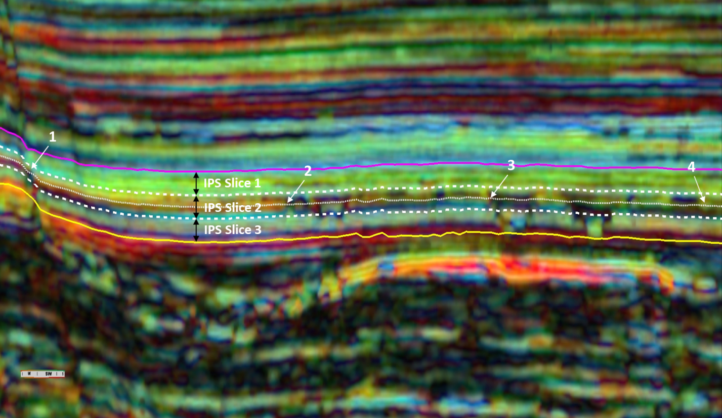
Figure 1 HDFD RGB blend along a section. The thin dotted line represents the centre horizon of IPS Slice 2, white dashed lines indicate the bounding horizons of the slice. The arrows are points of reference for the following images.
The iso-proportional attributes of a colour blend are calculated from the volumes that were used to set up the blend, in this case, the three magnitude volumes. The calculations will consider the values along each trace, between the top and base of each slice, from each input volumes. Let's examine the Maximum +ve Amplitude attribute: the algorithm takes the first traces of the 15 Hz, 35 Hz and 55 Hz magnitude volumes, analyses the interval between the top and base horizons (the two white dashed lines in this case), finds the strongest magnitude values, and in the last step, re-blends these three values using the same scaling as the original input RGB blend. This new colour value will be assigned to the centre horizon as a Maximum +ve Amplitude attribute, and the algorithm moves on to the next traces. Please note, that the maximum values along the same trace in the three input volumes are not necessarily located at the same vertical position. This attribute shows the mixture of the strongest responses within the slice.
The Maximum -ve Amplitude follows a similar approach. However, as there are no negative values in a magnitude volume, the attribute is calculated from the smallest values, from the weakest responses. This attribute is usually very dark.
The Maximum Peak to Trough Amplitude uses the difference between the highest and lowest magnitude values along each trace within the slice.
The RMS Energy calculates the root-mean-square value for each trace in the input magnitude volumes and re-blends them, as described above. In a sense, it is an average response of the analysed interval. Dominant Frequency attribute does not work with colour blends.
The following images show some of the iso-proportional attributes along the centre horizon (thin dotted line in Figure 1). In Figure 2 the actual RGB blend is draped over it, revealing a complex system of channels, mainly characterised by weaker responses than their surroundings.
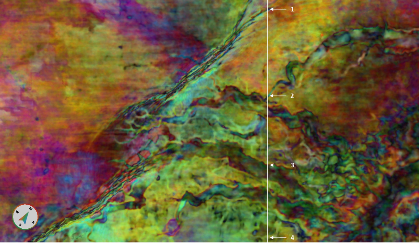
Figure 2 Horizon slice of the HDFD RGB blend draped over the centre horizon of IPS Slice 2. The white line indicates the location of the section in Figure 1.
Figure 3 shows the Maximum +ve Amplitude extracted from IPS Slice 2 and draped over the centre horizon of the slice. This attribute highlights the strongest responses within the slab: in a sense, this attribute reveals the dominant one of the three input frequencies within the slab. Please note that juxtaposed responses might originate from different vertical positions.
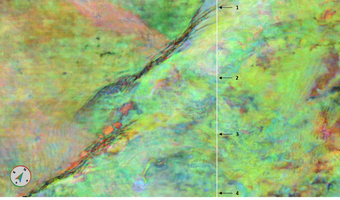
Figure 3 Maximum +ve Amplitude (Blend) attribute. This attribute highlights the strongest responses within the slab, regardless of their exact vertical position within the slab. The white line indicates the location of the section in Figure 1.
Figure 4 shows the RMS Energy attribute draped over the centre horizon of IPS Slice 2. This attribute could be interpreted as an average response of the slice. Although there are similarities with the image in Figure 3, this attribute shows a different picture, highlighting the dominant stratigraphic features of this unit, i.e. the channels.
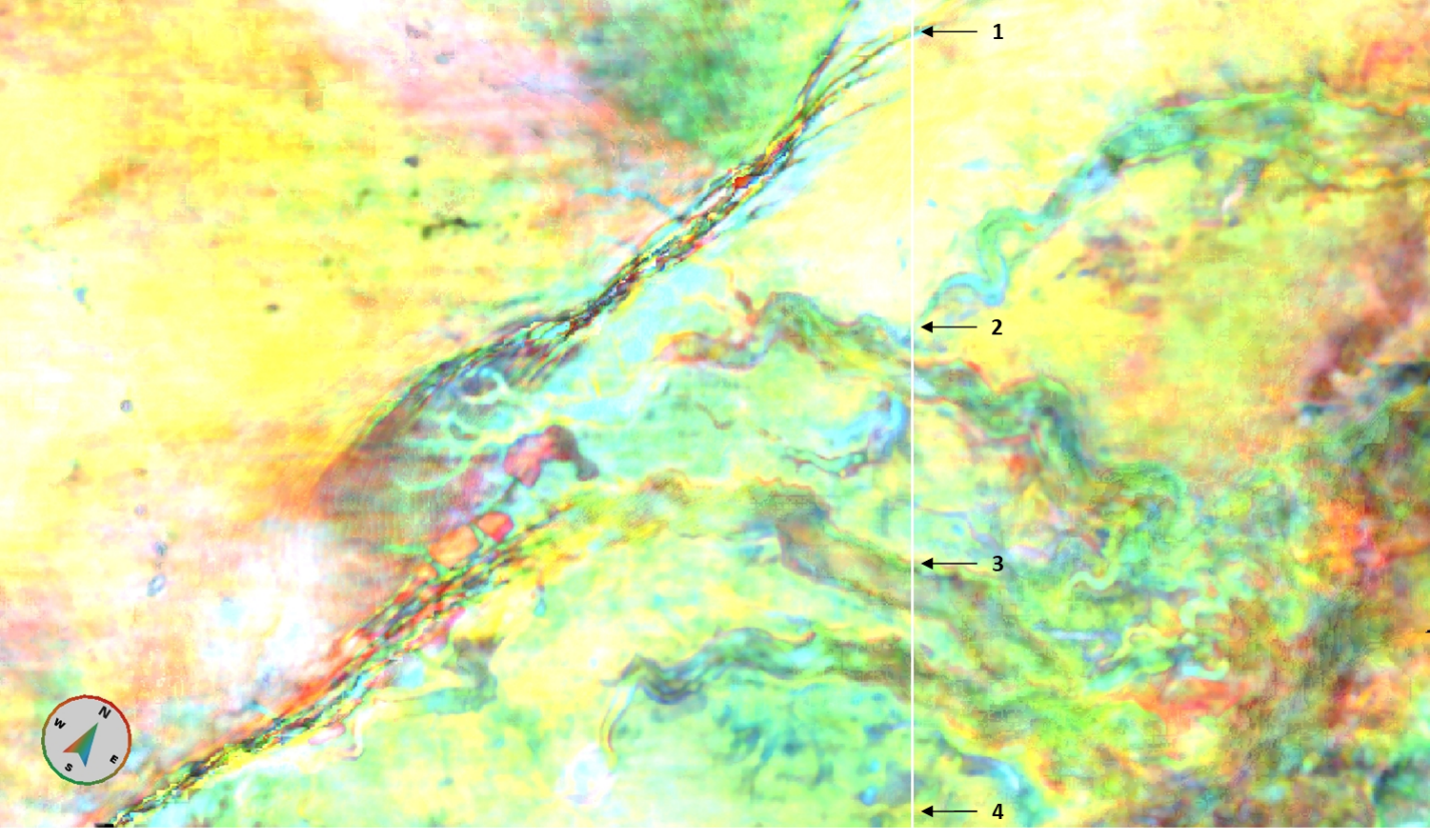
Figure 4 RMS Energy (Blend) attribute. The white line indicates the location of the section in Figure 1.
One might observe that the saturation level of Figure 4 is higher than that of the Maximum +ve Amplitude attribute (Figure 3). This might be a bit surprising, given that the RMS Energy is equally affected by the weak and the strong responses, and it is clear from Figures 1 and 2 that this interval is not characterised by strong responses only. The reason for this apparent contradiction is that the actual RMS values are multiplied by 2. This is current at the time this blog post is written, up to GeoTeric version 2017.2.1.1031. The adjusted RMS Energy attribute is shown in Figure 5 below. When compared to Figure 4, the colours are the same but are less saturated, as it would be expected, and the revealed features themselves are the same.
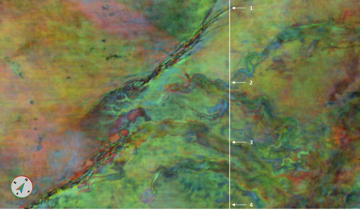
Figure 5 RMS Energy (Blend) attribute, adjusted for the scaling. The white line indicates the location of the section in Figure 1.
There is one more thing worth mentioning: when running the Iso-Proportional Slicing on a colour blend, all the visualisations within the tool honour the post-scale factors of the colour blend, i.e. if the post scaling is set high, we see brighter, more saturated colours in the preview screens of the IPS tool. However, the exported attributes do not reflect the post-scale factors, they use the default post-scale factor value of 1, therefore your actual attribute might show a different picture than its preview. In case you want the post-scale factors to be represented in the Iso-Proportional Attributes, there is a workaround - please contact us for more details.
