
One of the most popular applications of Geoteric’s Reveal module is the Fault Expression. Its example driven framework enables rapid optimisation and co-visualisation (CMY blending) of three independent edge attributes ensuring that faults of different sizes and seismic expressions are identified and detected with confidence.
A great value of the Fault Expression tool is that the effects of the different parameters can be immediately assessed: there is no need for extensive testing and comparisons, because after adjusting the filter footprints, the resulting changes are seen in the preview window. However, there is a set of parameters, which are hard wired and cannot be changed. These are the fault enhancement filters, mentioned in fine print in the Detect tab of Fault Expression. Switching between the different preview swatches, we see that the detected faults are different, even without changing the detection filter parameters. So, what do these numbers in the brackets mean?
In the first step of Fault Expression we can decide whether we would like fault detection to rely on a single attribute or a combination of Tensor, SO Semblance and Dip. In this blog post we will use a CMY blend, made of Dip 5x9 (cyan channel), SO Semblance 5x9 (magenta channel) and Tensor 5x9 (yellow channel).
Our Edge Detection algorithm is sensitive to sharp transitions of the edge attribute values, which in most cases represent the faults and fractures. However, there is always noise in the edge attributes, usually characterised by sudden changes in the attribute values. In order to avoid detection of these as edges, a spatial Gaussian filter is applied to suppress the random noise.
But before the filtering is applied, a transformation of the CMY blend is performed. The edge detection algorithm is only sensitive to the intensity of the edge responses and not to their colour, therefore the CMY colour blend is converted into a grey scale image, whereby the greyness represents the saturation of the colours: higher colour saturations will result in darker greys (Figure 1). This converted volume is added to the project, its default name in the Fault Expression tool’s output interface is cmy_greyscale.
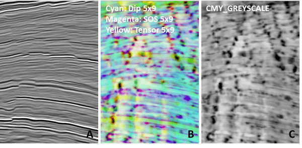 Figure 1 - The input seismic data (A), CMY blend of Dip, SO Semblance and Tensor (B) and the equivalent grey scale combined edge attribute. Colours are converted to grey based on their saturation.
After the colour-to-grey conversion is done, the fault enhancement calculations are performed in the background, the results of the calculations are not added to the Project Tree. As mentioned before, the purpose of this stage is to supress the noise and the stratigraphy related responses in the (combined) edge attribute and improve the continuity of the edges. A three-dimensional matrix is defined based on the enhancement parameters (e.g. 1x1x2 or 3x3x6). Each element in the matrix will represent a weight factor with which the value of a voxel in the given location will contribute to the enhanced edge attribute value in the centre of the filter. The numbers are sigma values, where sigma corresponds to the standard deviation of the Gaussian filter: a sigma=1 means that 68% of the energy of the filter is localised within ±1 voxels, while sigma=3 means that 68% of the energy of the filter is localised within ±3 voxels around the central voxel. Please note, that the three numbers in the filter’s description represent the sigma values along the x, y and z directions, the actual filter size is larger. The vertical sections in Figure 2 illustrate the effect of the Gaussian filter: in the original volume there is only one voxel with non-zero value, representing random noise. After enhancement, the energy of the noise is attenuated and distributed over several voxels (aka Gaussian blur), minimising the chance of detecting the noise as an edge. There are four swatches in the Detect panel of Fault Expression where the word Sharp is added: in these instances, an additional step, a type of minimum filtering is applied after enhancement to reduce the blurring.
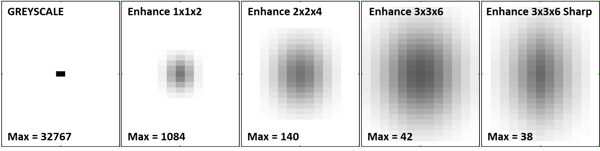
Figures 2 - Different Fault Enhancement filters applied to a volume with a single non-zero voxel, i.e. random noise. The energy of the random noise is attenuated and distributed, as shown in these vertical sections. Max values represent how the original 32767 changes with the different filters.
Figures 3 and 4 illustrate how the different enhancement filters affect the detected faults and their confidence levels. The three filters represent the first column of filters in the Detect panel. The enhancement attenuates the small-scale clutter in the edge attribute and smears the sub-horizontal stratigraphic boundaries, however, it also blurs some of the finer details, while enhancing the continuity of the stronger faults segments. As illustrated above, the Gaussian filtering distributes the energy of every voxel over a larger volume, thus decreasing the difference between the edge responses and their background values. Since the confidence level depends on the difference of the maximum edge attribute value and the average edge attribute value within the detection filter footprint (e.g. 9 or 17), stronger enhancement will lead to smaller confidence levels.
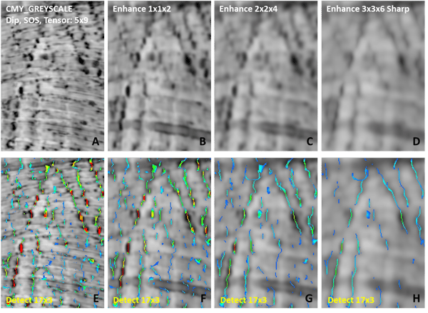
Figure 3 - Top row: a vertical section of the combined edge attribute of Figure 1 (A) and the same attribute after different fault enhancement filters have been applied (B, C and D). Bottom row: edge attribute from the top row co-visualised with the results of Fault Detect (17x3). The colour scales of the edge attributes and fault detect volumes are uniform. Note that with increasing enhancement filter sizes come decreasing fault significance values (for discussion see text above).

Figure 4 - Top row: a time slice of the combined edge attribute of Figure 1 (A) and the same attribute after different fault enhancement filters have been applied (B, C and D). Bottom row: edge attribute from the top row co-visualised with the results of Fault Detect (17x3). The colour scales of the edge attributes and fault detect volumes are uniform. Note that with increasing enhancement filter sizes come decreasing fault significance values (for discussion see text).
The flexibility of the Fault Expression tool enables the interpreters to rapidly test the different edge attributes and the fault detection parameters in order to optimise the workflow for their specific objectives. The hard-wired parameter sets represent the most frequently applied settings, and in most cases guarantee reliable fault detection results. However, if users would like to investigate other filter sizes, all these attributes and processes can be found in the Batch Processing Framework.
