

The aim of this workflow is to provide a more quantitative and analytical approach to understanding and distinguishing AVO anomalies.
Not all AVO anomalies show up as high amplitudes in the far stack. Instead, depending on the background geology, some AVO responses can be distinguished as a secondary trend in an overlying background. AVO gradient and intercept can be used to identify and distinguish these trends from a background response.
Background
This workflow is based on Shuey’s two term approximation of Zoeppritz’ reflectivity equations (Shuey, 1985). The approximation is valid for angles of incidence <30°, therefore very far and ultrafar stacks will be unsuitable inputs.
Shuey’s two-term approximation of the reflectivity equation is:
Shuey’s two-term approximation of the reflectivity equation is:
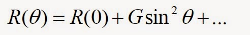
Where R is reflectivity at incidence angle θ. So plotting R versus sin2θ will give a straight line with gradient, G, and intercept, R(0) which is the ‘reflectivity at zero offset’.
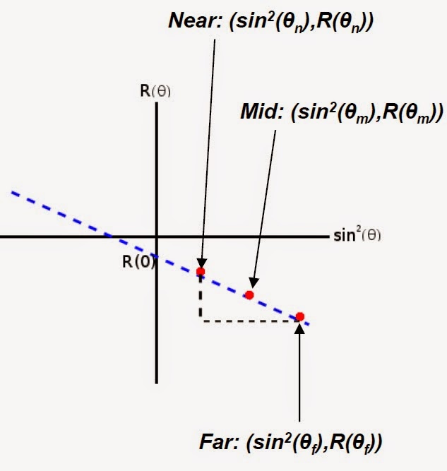
Plot of R vs sin2θ where a straight line between the angle stacks is identified
We have stacks at near, mid and far offsets, so if we know the central angles we can estimate the gradient using the following formulas:
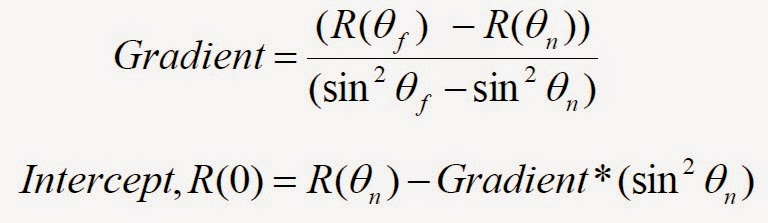
Each angle stack has normally an angular range (for instance 5° to 15°) which for the purpose of this workflow will be approximated to the central angle (i.e. 10°). This is a source of uncertainty in the resulting gradient and intercept volumes.
Another source of uncertainty is the fact that we are using a linear approximation to calculate the gradient from the near and far, instead of using a least squares calculation.
Another source of uncertainty is the fact that we are using a linear approximation to calculate the gradient from the near and far, instead of using a least squares calculation.
The workflow
In Geoteric, we can use the Parser to create the Gradient and Intercept volumes based on two angle stacks, normally near and far. The Parser can be found in Processes & Workflows > Processes > Volume Maths > Parser.
To calculate the Gradient volume we can use the expression:
(im2-im1)/((sin(θf*pi/180))^2-(sin(θn *pi/180))^2)
Where im1=near stack reflectivity, im2=far stack reflectivity. θf and θn need to be replaced by the central angle of the far and near stacks.
If the output volume is clipped (check the histogram using Opacity), you may need to re-run the parser applying a scale factor to keep the data within your dynamic range:
((im2-im1)/((sin( θf *pi/180))^2-(sin( θn *pi/180))^2))/scale
The intercept volume can be calculated using the expression:
im1-(im2*((sin(θn*pi/180))^2))
Where im1=near stack reflectivity, im2=gradient. θn needs to be replaced by the central angle of the near stack.
If the gradient volume was scaled to avoid clipping, the intercept volume expression will need to be scaled using the same factor:
If the gradient volume was scaled to avoid clipping, the intercept volume expression will need to be scaled using the same factor:
(im1/scale)-(im2*((sin(θn*pi/180))^2))
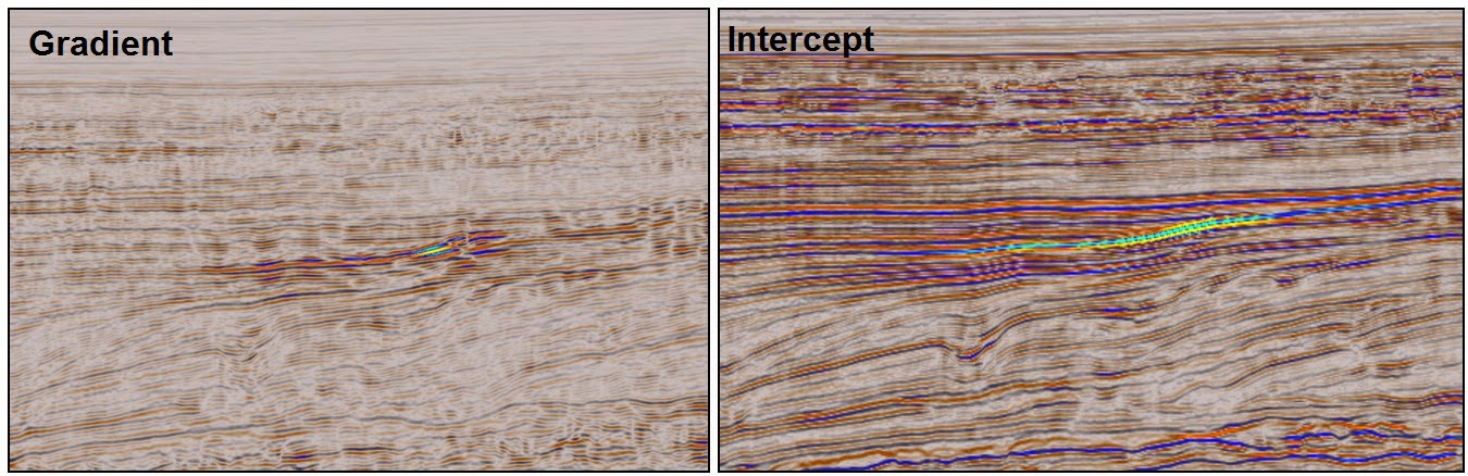 Gradient and Intercept volumes calculated on the Rosewall-Calliance 3D dataset (NW shelf Australia)
The scatterplot
The scatterplot available within the IFC+ tool can be used to crossplot sample areas on a gradient and intercept crossplot and identify potential fluid anomalies.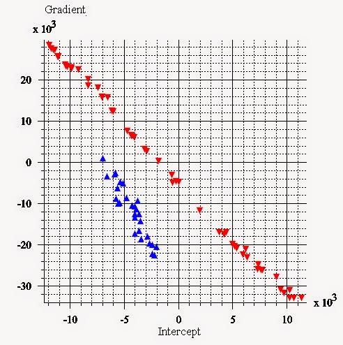 Gradient vs Intercept scatterplot showing a background area (red class) and a class III anomaly area (blue class)
See here for part 1, part 2, part 4, and part 5 in this series where we will cover how to create the AVO product and Reflection coefficient difference volumes and Scaled reflectivity.
