

RGB Blends of Frequency Decomposition results are very powerful in revealing fine details of the subsurface, but the amount of information that can be extracted from such blends depends on which band-limited response magnitude volumes are used as an input. Selection of the right frequencies depends on the interval, amount of detail and objective of the analysis.
Let us start with a quick overview of the frequency decomposition algorithms Geoteric offers. The Constant Bandwidth algorithm uses a constant filter length – defined by the lowest central frequency set by the user – and offers the highest frequency resolution, but it is the weakest when it comes to vertical resolving power. The Constant Q algorithm utilises a variable filter length, thus a variable bandwidth, and has a better vertical resolution than the previous approach. The best vertical resolution is provided by the High Definition Frequency Decomposition (HDFD). The frequency and temporal (vertical) resolutions are linked through the uncertainty principle: increase in one unavoidably leads to a decrease in the other. More details about these frequency decomposition methods and how to use them are found in previous blog posts:
There are several scenarios for using Frequency Decomposition and RGB Blends to bring out geologic data. The first case is when we are in a total reconnaissance mode, i.e. we have a new data set and would like to get a first overview of the different geological features. The quickest way to a useful frequency decomposition colour blend is to use the Exponential Constant Q option in the Frequency Decomposition workflow. A reference time slice should be chosen to reflect the potentially most prospective interval. Generate a spectrum along this time slice, then modify the minimum and maximum frequencies so that they correspond to frequency values where the power spectrum reaches 30-50% of its peak value (note that the vertical axis of the graph is divided into 10 equal intervals), see Figure 1. In most cases four bins will be sufficient, however, in case of broadband data this value might have to be increased to ensure that adequate overlap is provided between the filters.
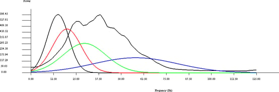
Figure 1: Minimum frequency is set to 15 Hz while the maximum frequency is set to 58 Hz (with 19.9 Hz and 29.6 Hz between them). The four different filters (bins) provide adequate overlap.
It can be beneficial to create two colour blends: one using the lowest three bins, while the other using the higher frequencies. This can guarantee that most of the frequency responses are covered and accounted for in the reconnaissance blends. Figure 2 is the reflectivity data that will be used in this example. The data is from the Parihaka 3D, offshore New Zealand. This is a time slice of 1300ms depicting a channel system coming in from the east. In Figure 3 and 4, are the two reconnaissance colour blends. Figure 3, blend of the lowest three frequencies and the higher frequencies in figure 4.
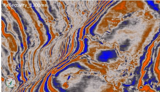
Figure 2: Reflectivity data at 1300ms, illustrating channel system of interest.
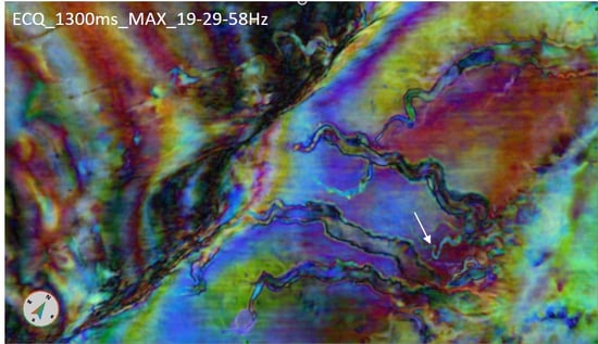
Figure 3: Uniform Constant Q Frequency Decomposition RGB Blend using the higher frequencies (19-29-58Hz), white arrow pointing to channels of interest.
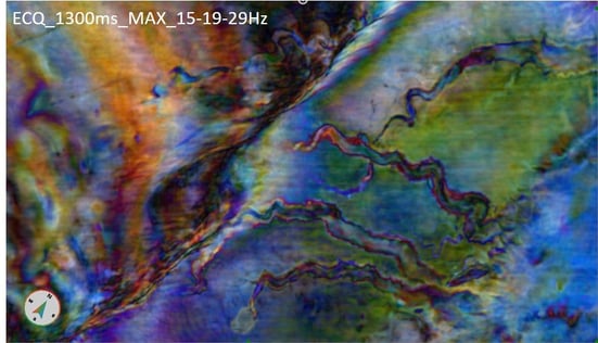
Figure 4 Uniform Constant Q Frequency Decomposition RGB Blend using the lowest frequencies, 15-19-29Hz.
Once an object of interest has been identified, the combined frequencies can be selected in a more focused manner. Take for example the thin channel highlighted by the white arrow in Figure 4. Its cyan colour indicate that it is probably not present in the 19 Hz magnitude volume, but can be found in both the 29 and the 58 Hz magnitude volumes. We can further fine tune this information with the help of the spectral attributes, which are calculated by the Frequency decomposition tool. In this example we’ll use the Mode volume, which can be interpreted as the dominant frequency at every single voxel. Figure 5 shows the same time slice, 1300ms, from the Mode volume, calculated using Constant Bandwidth approach, with 15 bins between 12.5 and 60 Hz. Please note, that in the output volume the frequency values are scaled, depending on the data type: in 16-bit data the scaling factor is 100 (12.5 Hz = 1250), while in 32-bit data it is 1000 (12.5 Hz = 12500).
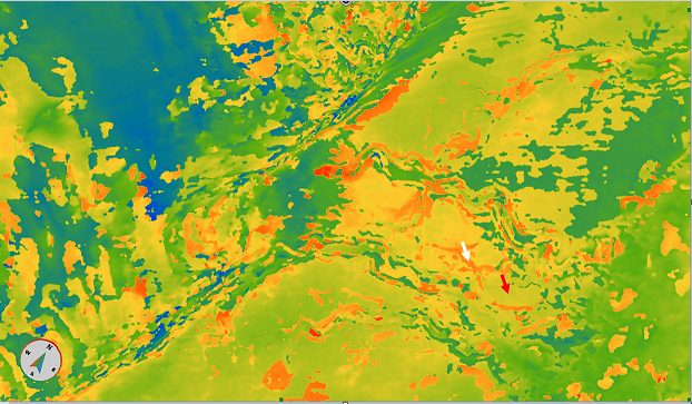
Figure 5: Mode (dominant) frequency along the time slice (dark blue = 12.5 Hz; red = 60 Hz). The small channel changes dominant frequency, from mid-thirties (red arrow) to high forties (white arrow).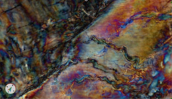
Figure 6 Blend of 39, 43 and 46 Hz, Constant Bandwidth method. The thin channel can be detected along a significant length, and the variation in its dominant frequency can also be studied
Now that we know the dominant frequency values at this level, we can focus the frequency blend to highlight the thin and narrow channel as much as possible. Figure 6 shows a colour blend of 39, 43 and 46 Hz, calculated using the Constant Bandwidth approach. Please remember, that this method gives the highest frequency resolution, however, it has the most significant vertical smearing. It is very likely, that not all segments of the channel seen in Figure 6 are actually located at the depth of the time slice.
Another way to optimize the frequencies for a colour blend is to visually compare the different frequency magnitude responses in the Data Preview window of the Frequency Decomposition tool, see Figure 7. Viewing the different magnitude volumes allows the interpreter to compare the different response strengths of a geological feature at different frequencies. For an exact comparison please make sure, that the colour compression (Minimum Value and Maximum Value) is the same for every slice
.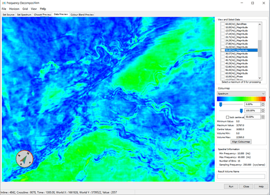
Figure 7 The Data Preview window allows for a direct comparison of the different response strengths at different central frequencies.
To image the thin channels with their correct vertical localization, the High Definition Frequency Decomposition should be used. This tool has a different way of selecting the desired frequencies. After identifying the target feature, select a representative inline or crossline across it and use it in the HDFD tool. Set the spectrum extraction window (the green sliding arrow on the right-hand side of the tool) so that it has the target feature in the centre (Figure 8).
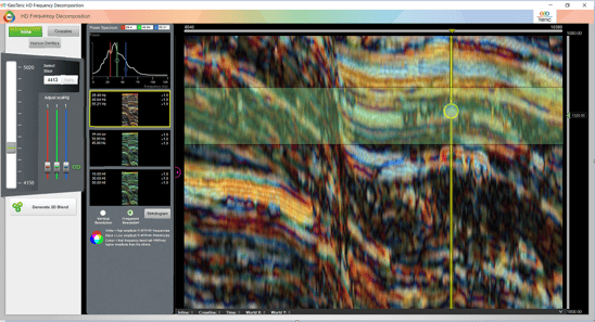
Figure 8 Select a representative inline or crossline and adjust the spectrum calculation window.
The Spectrogram button opens a new window (Figure 9), and, at the same time, displays a vertical yellow line with a circle on it in the main HDFD window. By dragging the circle to the feature of interest we can start analysing the HDFD trace spectrogram. This spectrogram is calculated from the reconstructed trace along the yellow line (in this case it is inline 4413, crossline 9696). The resolved seismic events are represented by the narrow zones of green-to-red colour, whose lateral extent represents the uncertainty in their frequency. The position of red, green and blue lines can be adjusted to cover the frequency interval where the highest energy of the response is concentrated. Using the Spectrogram, we can set the three frequencies to best represent the investigated target.
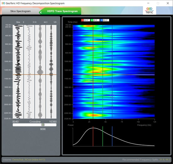
Figure 9 HDFD Trace Spectrogram along the yellow line in the main HDFD window, Figure 8. The horizontal brown line represents the position of the yellow circle. The red, green and blue frequencies can be adjusted to cover the strongest frequency response of the analysed feature.
The resulting HDFD magnitude volumes, calculated with the Frequency Resolution option, can be blended either by the HDFD tool or by using the Tools -> New Colour Blend option. The latter gives an opportunity to optimise the scaling factors for a horizon, which in many cases provides a better image of the targeted geological features. As Figure 10 shows, the superior vertical localisation power of HDFD confirms that the thin channel, discussed in Figure 6 does not run fully along this time slice
.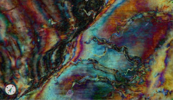
Figure 10 Blend of 24.5, 37.5 and 51.6 Hz, High Definition Frequency Decomposition, Frequency resolution option.
