In order to get a more accurate understanding of reservoir extents, attributes can be segmented based on petrophysical cutoffs, and geobodies can be created from segmented volumes using the Parser tool.
The Parser is the ultimate process to edit or combine volumes. It gives the user complete control over how the data is combined. The Parser is a volume base calculator, an arithmetic expression is applied on a per voxel basis across one or more input volumes.
The only inputs to the Parser are the volumes and the mathematical expression. The volumes are referenced as im1 (image 1) to imN in the expression. If there are two or more volumes, they will be referenced as im1, im2, etc. The image numbering is related to the order they are selected, the first volume in the Selected column is im1. The expression follows that of a standard mathematical expression.
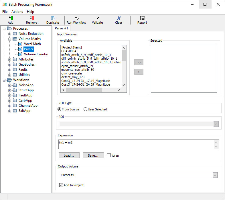
The mathematical expressions can be as simple as im1 + im2 or more sophisticated with logical operators. In the help file we can find a wealth of information and parser expressions examples.
A good resource are the pre written "parser expressions" available in .txt format. Here's a list of some of the files provided:
Combination/ arithmetic_combo_divide_s16_s32_template.txt
Combination/body_and_fault_s32.txt
Scaling/data_scaling_s16_s32_template.txt
Segmentation/facies_map_template.txt
Combination/general_invert_second_s16_s32_template.txt
Analysis/median_of_three.txt
Analysis/multiple_cluster_analysis_template.txt
Scaling/non_linear_scaling_s16_s32_template.txt
Analysis/single_cluster_analysis_s16_s32_template.txt
Analysis/real_azimuth_32bit.txt
The Parser expression files will have been loaded on installation of GeoTeric in the *installation directory*\help\libs\parser folder. On the help file you will find an explanation of what each expression does and few examples of resulting volumes.
Using the Parser is a very effective way to segment data based on specific threshold attribute values, this is particularly useful when working with attribute and inversion volumes in order to characterize a reservoir.
In the figure below, Geoteric's workflow was used to identify the structure of interest, in this case a turbidite channel.
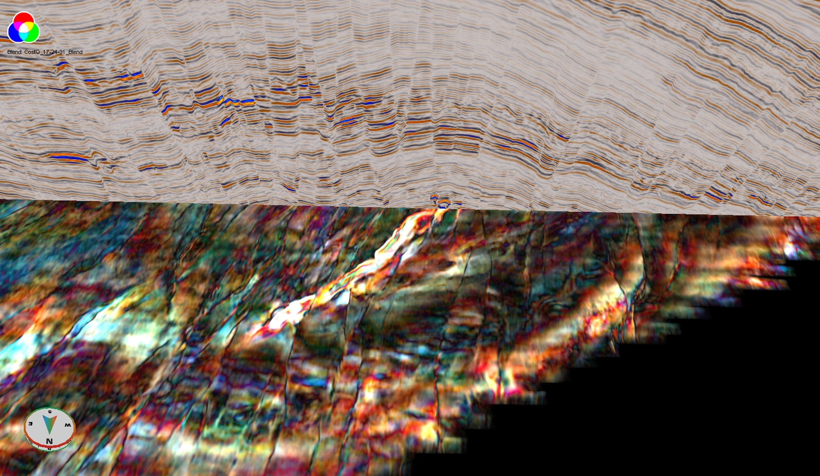
The Frequency Decomposition results highlight the channel's full structure. If further characterization of the reservoir is to be achieved the inversion volumes can be used to determine different lithologies, fluids and best porosity. The threshold values for the individual attributes can be obtained via a petrophysical analysis or using the scatterplot tool. Once we have the values ranges for the attributes, a parser expression can be written in order to produce a geobody when all the conditions are met. The parser expression would be:
((im1>T1 & im1<T2) & (im2>=T3 & im2<T4) & (im3>T5 & im3<=T6))*C1
Im1 - Attribute 1
Im2 - Attribute 2
Im3 - Attribute 3
T1 - Lower threshold values for attribute 1
T2 - Upper threshold values for attribute 1
T3 - Lower threshold values for attribute 2
T4 - Upper threshold values for attribute 2
T5 - Lower threshold values for attribute 3
T6 - Upper threshold values for attribute 4
C1 - New values for the voxels, this value will dictate position of the geobody on the color bar, in other words it will dictate its color.
In this example, the value of im1 is greater that T1 and less than T2. The value of im2 is greater than or equal to T3 and less than T4, etc. All of the voxels that adhere to this equation will then be given the voxel value of C1. If a reservoir is characterized by a certain range of acoustic impedance values, Poisson Ratio values and porosity values, when all of these conditions are true the voxels will have a value of C1 and all other voxels will be replaced with zero.
This particular combination of inversion attributes will identify the channels "sweet spot" in terms of rock properties (image below).
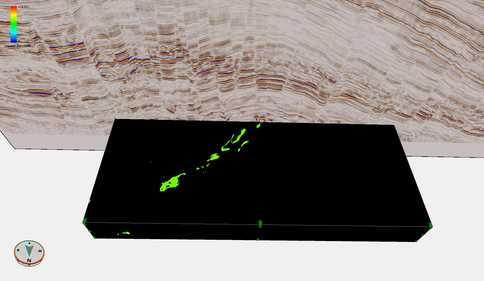
The resultant geobody of the parser equation displayed in 3D:
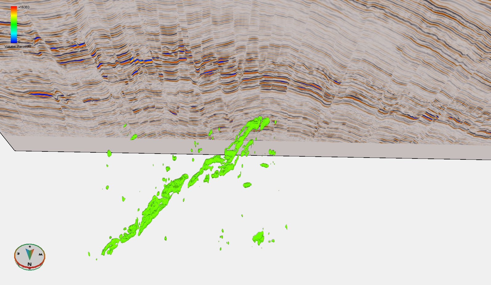
In the figure above, the opacity curve was used to remove all the zeros from the display, leaving the geobody rendered in 3D. This way we can have a better understanding of the lateral distribution and connectivity of these bodies.
If the Parser expression is changed slightly we can incorporate the information of a fourth volume. The three first attributes are used to segment the data, the generated body can them be populated with the information of the forth attribute.
((im1>T1 & im1<T2) & (im2>=T3 & im2<T4) & (im3>T5 & im3<=T6))*im4
Im1 - Attribute 1
Im2 - Attribute 2
Im3 - Attribute 3
Im4 - Attribute 4
T1 - Lower threshold values for attribute 1
T2 - Upper threshold values for attribute 1
T3 - Lower threshold values for attribute 2
T4 - Upper threshold values for attribute 2
T5 - Lower threshold values for attribute 3
T6 - Upper threshold values for attribute 4
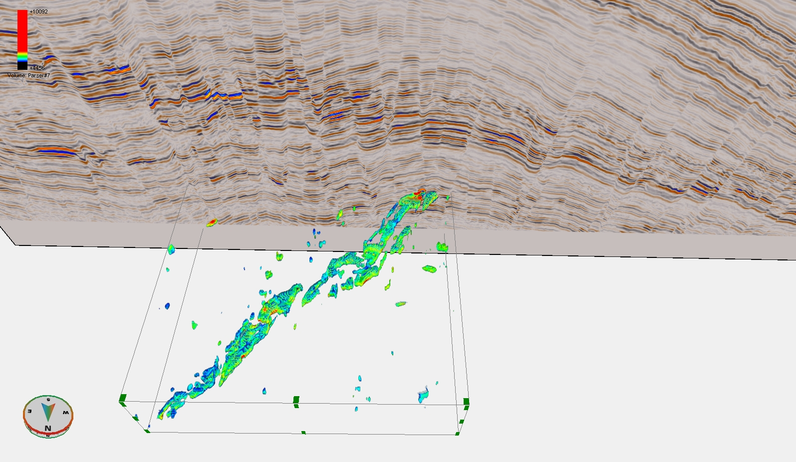
The figure above uses the same geobody, now with a fourth attribute generated within the geobody. This helps to further characterize the areas of interest and is a visually informative way to show information from four different attributes.
This workflow can be applied at different times of the life cycle of a prospect: during exploration for lead maturation, when only a few attribute values are known. During field development, and reservoir characterization when more wells have been drilled and the attributes can be more constrained for better well placement and during production for reservoir monitoring.
This tool provides a fast and simple method for identifying the extents and geometries of prospects based on your prerequisits, allowing you utilise all of the available data and attributes, and highlighting your sweet spot.
