

The Scatterplot in the IFC+ tool can be used to investigate the tuning thickness of localised areas in a data set. The tuning curves are displayed using the Terrace Amplitude and Terrace Thickness volumes. This can be calculated within the batch processor - Processes > Attributes > Trace Attributes > Attributes > Terrace
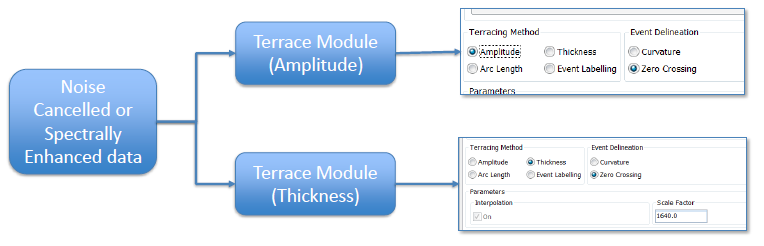
The input for the workflow is a data conditioned volume, either Noise Cancelled or Spectrally Enhanced.
Re-scaling
the Thickness volume
The Thickness volume is scaled to use the full dynamic range of the data so the values don’t have geological significance. We need to remove the scale factor and also multiply by the sample rate of the data to turn the thickness values into milliseconds (ms). This is calculated in the Parser using the scale factor that is automatically calculated in the Terrace module and is available in the volume notes.
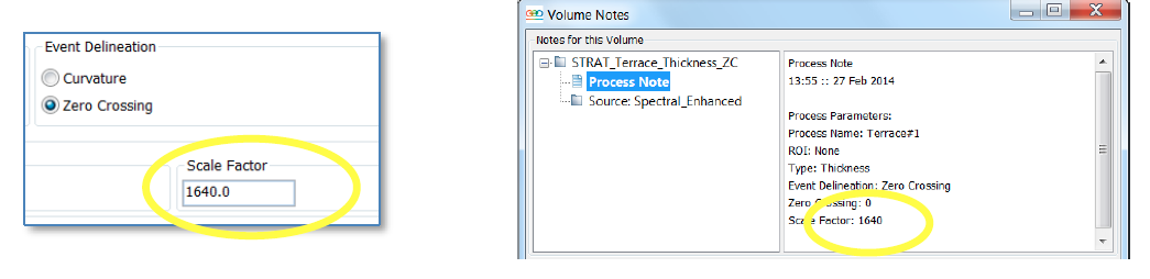
The volume notes can be found by right clicking on the volume and selecting ‘volume notes’
Parser Equation: (im1/scale_factor)*sample_rate
For the example above the equation would be: (im1/1640)*4 The output values will now be the reflector thickness in ms.
Calculating the Absolute value
The Terrace module outputs positive and negative values for the peak and trough amplitude / thickness values. To create a tuning curve it is preferable to have positive values only. Calculating the absolute value of the Terrace attributes using the Parser will make all the negative values positive alongside the values that are already positive.
This is achieved in the Parser with the following expression:
abs(im1)
This should be run on the Terrace Amplitude volume and the re-scaled Terrace Thickness volume.
Using the Scatterplot to create the Tuning curve
- The Scatterplot is part of the IFC+ tool and enables the user to crossplot different attribute values within a defined region.
- The regions are defined by drawing polygons on any volume (or RGB blend) in the main IFC+ tool.
- The attributes that are crossploted can be different to those used to draw the polygon on (and/or the sources for the classification).
- This allows users to compare the tuning curves of different areas which can be identified by other attributes (such as RGB blends).
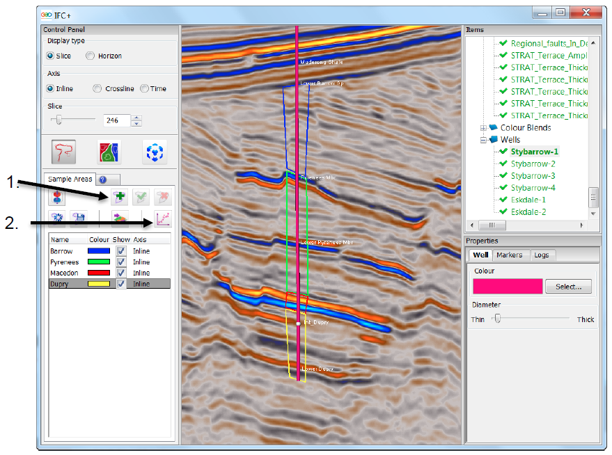
Step 1, define the areas in the IFC+ tool by drawing sample areas which represent the zones of interest.
In the example below different zones down a well have been selected.
Step 2, send the sample areas to the Scatterplot. Multiple sample areas can be sent to the same Scatterplot or they can be sent to individual Scatterplots.
Select the Absolute_ Thickness volume as the first input and the Absolute_ Amplitude volume as the second input in the scatterplot tool.
Tuning thickness in metres is calculated by taking the Tuning Thickness in ms, divide by 1000 to put into seconds, divide by 2 to get OWT rather than TWT, then multiply by your known velocity.
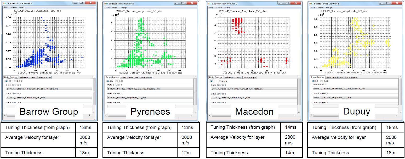
As we can see in the above examples the tuning thickness increases with depth from 13m in the Barrow to 16m in the Dupuy.
.
