

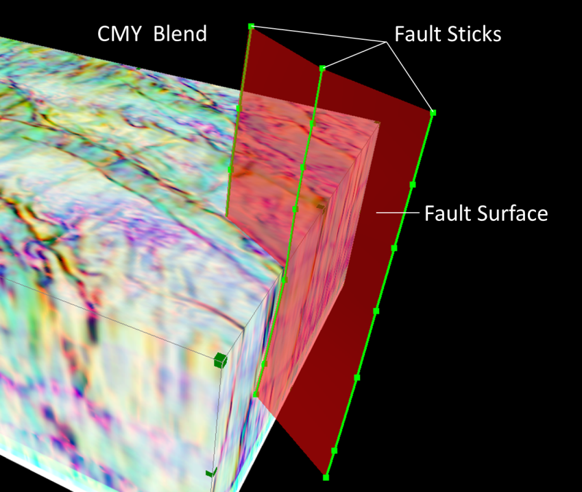
The Fault Interpretation and Interactive Fault Slicing tools allow for interpretation on CMY blends, RGB blends, or any attribute volume on both inline/crossline slices and time slices in the 3D viewer, providing a huge degree of freedom and capability to provide the optimal fault image to pick on. The resulting faults can be used in novel and unique ways to gain a greater insight into your seismic data
The interpretation itself is achieved through fault stick picking, and the generation of surfaces based on those picks. To initiate the process, navigate to either the ‘Interpretation’ drop down in the refreshed 2014.2 toolbar, or click on the ‘Faults’ folder in the project tree, and in either case select ‘Enable Fault Picking’.
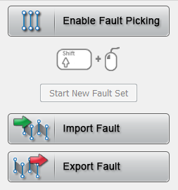
This begins a new set of fault sticks. Each set can be converted to a fault surface. To pick, make sure the display is in Pointer/Pick mode, and then holding down the Shift key, left-click on a volume or blend to add points to a fault stick. To start a new stick, release the Shiftkey, adjust the position of the slice or volume, then hold Shift again to resume picking. All of the display and probe controls continue to work in Fault Picking mode. To start a new fault stick set at any time, click ‘Start New Fault Set’.
Tip
: More complex fault stick sets will make it harder for the software to generate smooth fault surfaces. Regularly spaced, parallel fault sticks will make it easiest.
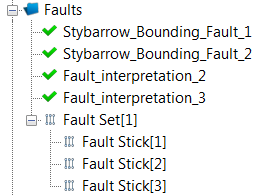
The Faults folder will then be populated with ‘Fault Sets’ containing the picked fault sticks. Within each Fault Set, you can access the individual sticks and delete or rename accordingly. To convert a Fault Set to a continuous, smooth fault surface, just right click on the set of interest and choose ‘Create Surface’.
The created surfaces can be cached and visualised by double clicking, as with other project items. The properties panel for a fault provides three tabs:
- Mode: Change the visualization properties. Note that by selecting ‘Data Mapped’, volumes and colour blends can be projected onto the fault plane, and have full colour bar control.
- Tip: To display a smoother fault surface, move the Crease Angle slider all the way to ‘Diffuse’
- Overlay: Select ‘Activate’ to display the fault plane as a line intersection on any vizualised volume in the 3D viewer.
- Interactive Fault Slicing: This mode enables you to move the fault in real-time in 3D, and dissect data volumes in a very powerful way as explained below:
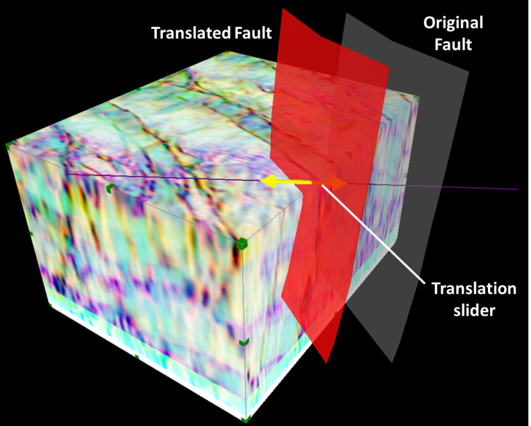
On this tab, click 'Enable Fault Translation' and an arrow control will appear, normal to the mean centre of the fault surface. Drag this arrow in Pointer / Pick mode, and the fault surface will slide along the line normal to the fault. '3D Normal' does this entirely in 3D, whereas '2D Lateral' locks the translation to the XY plane. 'Show Original' will display a ghost of the original fault and deactivating Fault Translation will reset the fault to its original position. Click 'Save as New Fault' to create a shifted clone of the original.
Any mapped volume or blend will also update with the translated fault, making this an excellent tool for investigating throw and juxtaposition of stratigraphic units across a fault:
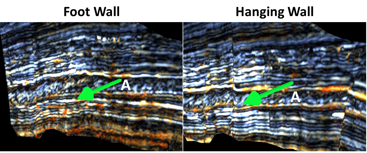 |
In the above images, a fault translation enabled on a an HDFD colour blend mapped, has been shifted to either side of the original fault plane. We can clearly see that unit A of prograding clinoforms is at a higher position in the footwall than the hanging wall, instantly confirming this to be a normal fault. The throw suggests the unit remains in juxtaposition with itself across the fault.
Finally, picked faults can be exported from GeoTeric by clicking on the 'Faults' folder. At present, the supported format is GOCAD Tsurf.
