A common question with regards to RGB colour blends is “what do the colours show me” or “is there a way to show other areas with this response”. In this post we will look at how using the Mean frequency can be used to address these questions.
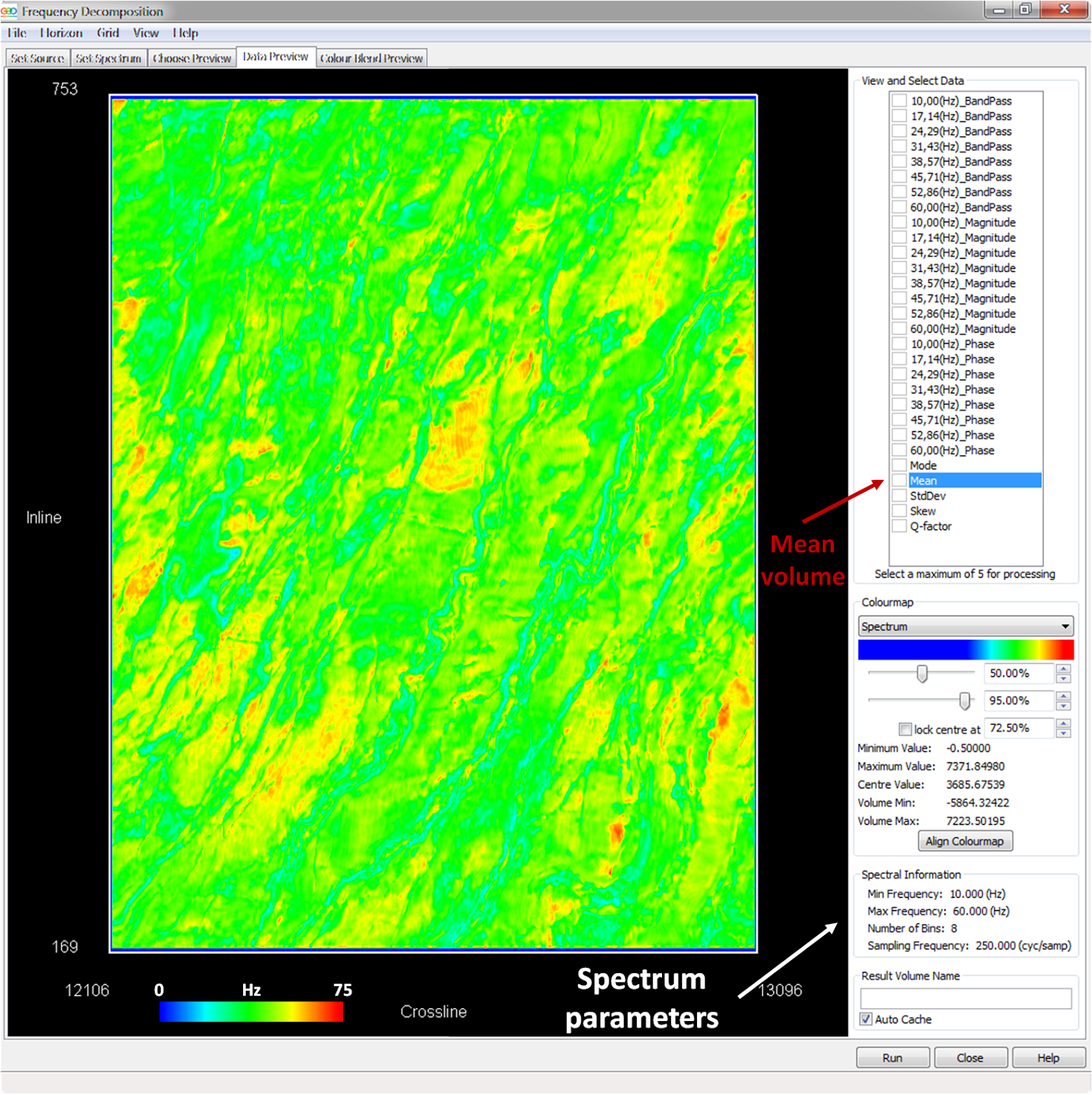
The Mean frequency can be calculated in the frequency decomposition workflow and previewed using the normal preview. It is important to remember the Mean is calculated with the same parameters as the standard frequency decomposition volumes (Bandpass, Magnitude and Phase). Therefore, using the Constant Bandwidth method will produce a higher frequency resolution over a larger vertical window and the Constant Q method will have lower frequency resolution but higher vertical resolution.
With the Mean and Frequency Decomposition blend computed it is possible to try and identify different blend response against the frequency response. This can be very useful in identifying changes in sedimentation, fluid fill and porosity.
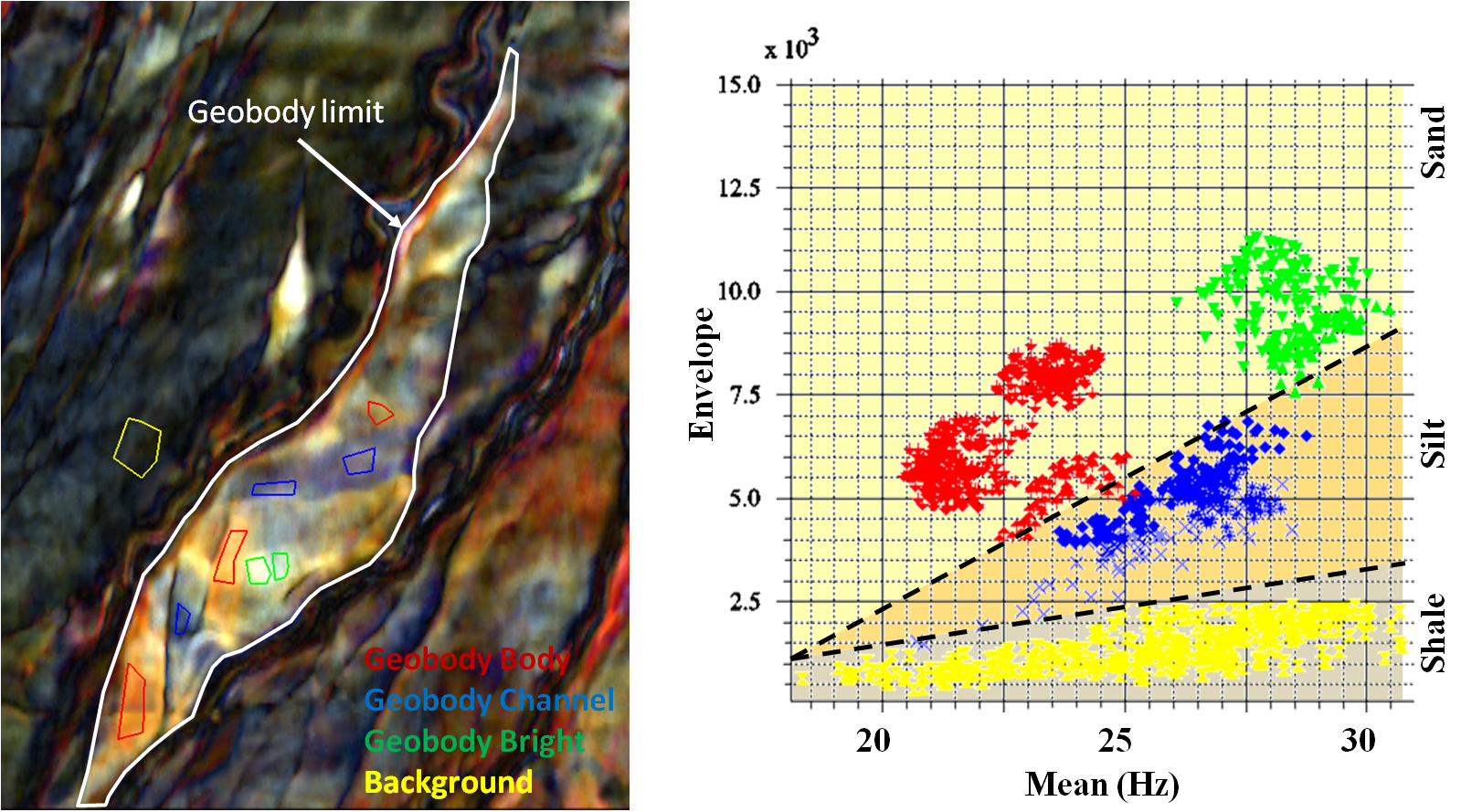
The Mean volumes can be used to help analyses of Frequency Decomposition blends in the Interactive Facies Classification tool (IFC+). By selecting a number of sample areas to identify different parts of a feature, it is possible to classify the geological event. In this case the feature below has been separated into 4 component parts; body of event (red sample areas), internal channels (blue sample areas), bright sections (green sample areas) and background (yellow sample areas). It is important to remember that a constant scaling factor has been applied to the frequency during the frequency decomposition process. For 16Bit data the scale factor is 10,000 and for 32Bit data it is 100,000.
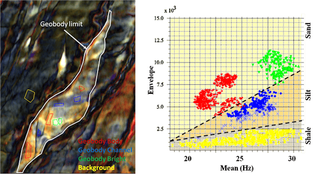
Each of these sample areas can then be imported to the crossplot function within the IFC+ tool with the Mean plotted against Envelope. Envelope is a useful volume to plot frequency against as they both show independent components of the seismic trace (Envelope = reflector strength, Mean = frequency). Once loaded into the crossplot tool it may be possible to identify different areas of the feature by different frequency responses. In the above example it is possible to differentiate the background (yellow) from the channel (blue) and reservoir (red and green) samples. The interpretation of the feature suggests the background is shale bearing, the channel events within the feature are silt based and the main body of the feature and the bright spots are sandstones of varying thickness. With this geological understanding the crossplot can be further separated into these component sections.
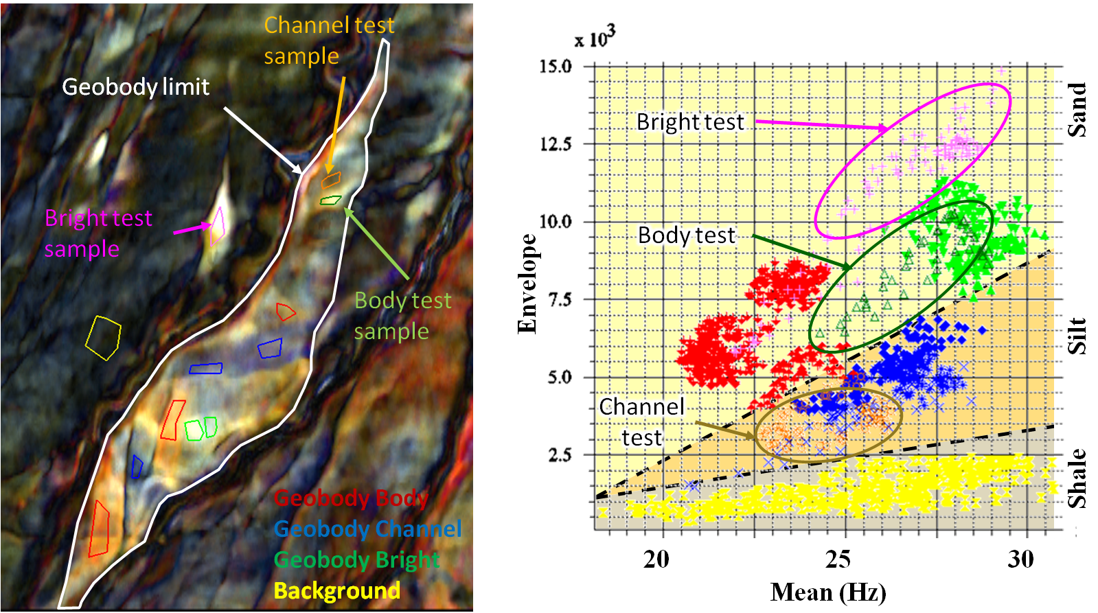
Taking these results forward can be achieved by collecting more sample areas either in different locations of the feature to confirm the change in sedimentation/fluid fil/porosity or by selecting more sample points in different features to de-risk prospects. In the below example 3 “test” sample areas have been selected in an attempt to distinguish the geology of the northern section of the feature and a neighbouring satellite feature.
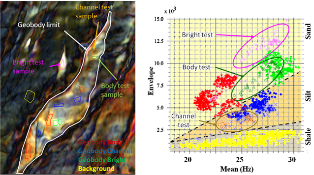
The results from the test samples show the satellite area (pink) which has a bright response in the blend matches well with the bright samples within the main feature. From this we can conclude it may have a similar geological composition/fluid fill/porosity. Further correlation can be made between the northern extreme of the feature where both body (dark green) and channel (orange) test samples were collected and again match up with our earlier analysis. By running this style of analysis you may be able to better understand sediment distribution and reservoir quality within a feature to help make accurate interpretations for model building or STOOIP calculations.
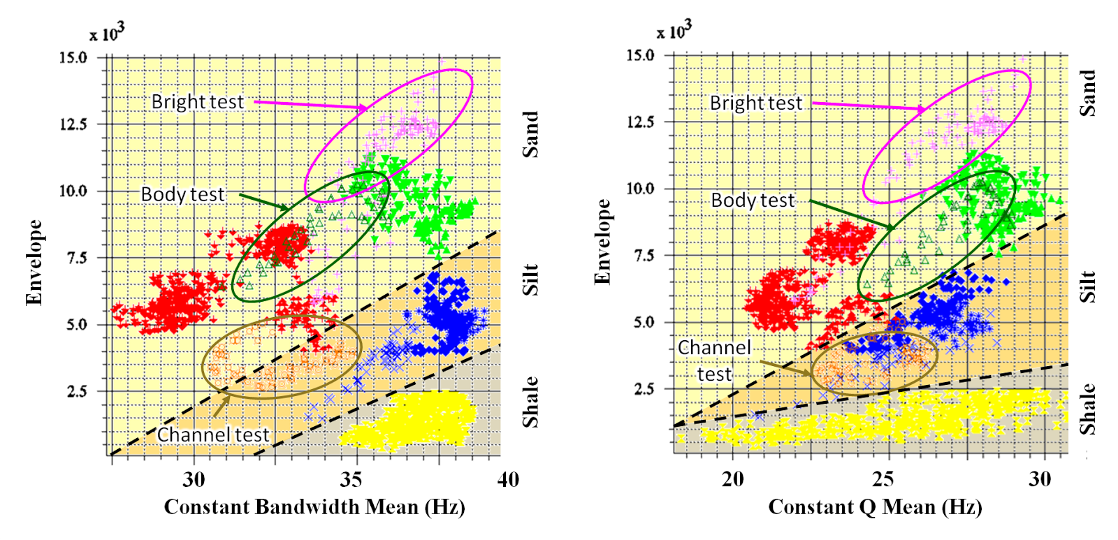
This process can be replicated using different blending methods (Constant Bandwidth vs Constant Q) and Mean, as shown below. By changing the input and its parameters on the x-axis the charts may look quite different, but differentiations between the different environments can still be made.
Another way this analysis can be used is by identifying individual areas and their respective frequency response, such as the silty sediments in the Constant Q methods which have a frequency response between 23-26Hz. This is extremely useful if your hydrocarbon bearing reservoir is giving a distinctive frequency response.
Both of these methods assist in interpreting differences within a geological anomaly and locating other areas in a volume that may have a similar response to one that is already defined.