This is an extended workflow from an earlier Tuning Curve Analysis blog post where it shows how to generate a Tuning Curve using Terrace Amplitude and Terrace Thickness. The input for Terrace Amplitude and Terrace Thickness should be phase rotated -90 degree or Quadrature attributes of your seismic.
Now, we want to create a Tuning classification volume based on the Tuning Curve that was created.
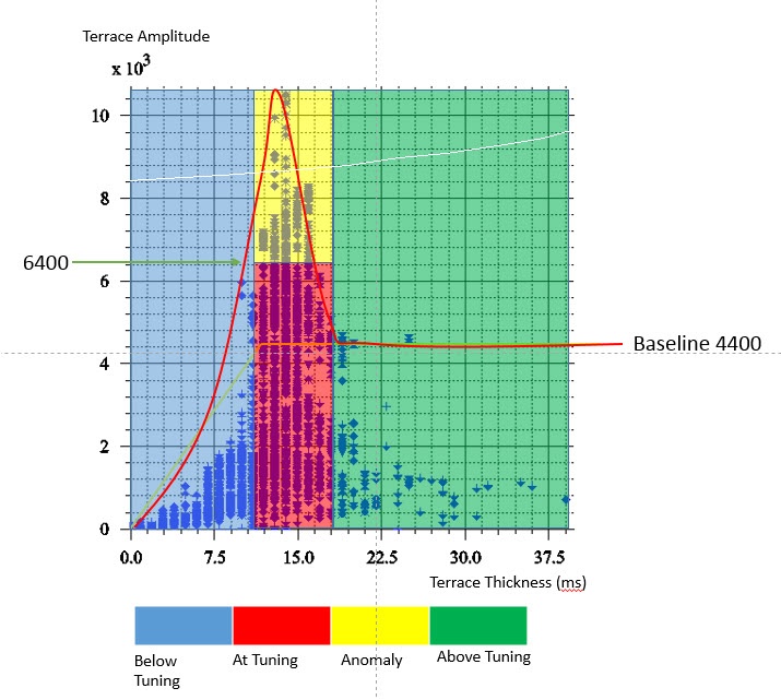
Above is an example of a crossplot between Terrace Amplitude and Terrace Thickness. First a baseline is defined which represents the maximum amplitude values expected if no tuning had taken place (yellow line). Points with amplitude values above the baseline are those thought to be boosted by tuning. The baseline has a constant amplitude value at thicknesses greater than or at tuning thickness and then slopes to zero below tuning thickness. The turning curve (red line) encompasses the majority of points, including the high amplitude values thought to be boosted as the result of tuning (reference to Brown et al. 1984,1986).
The resulting crossplot reveals that the tuning thickness is in the range of 11-18ms, below tuning is less than 11ms and above tuning is more than 18ms. Based in this information, using the Terrace Thickness as an input, we could create a volume that highlight the areas which is below Tuning, at Tuning and above Tuning using the Parser. Each category will be denoted by a value.
2=areas of data where thickness is below tuning thickness
4=areas of data where thickness is at tuning thickness
6=areas of data where thickness is above tuning thickness
The parser equation will read as:
((im1>0)&(im1<11))*2 + ((im1>=11)&(im1<=18))*4 + (im1>18)*6
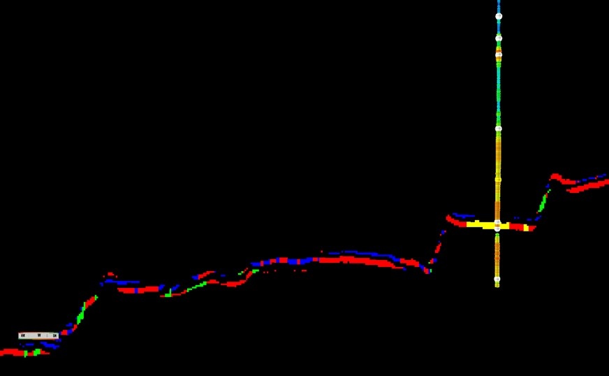
This should then create a classification volume similar to example below.
If you happen to do a forward modelling to see the effect of fluid to your amplitude and how much percentage it contribute to the amplitude within the at Tuning range, we could further classify our at Tuning areas into areas of tuning amplitude and anomalies. From our model, we approximate that 45 percent from the value of the baseline,4200 that is 6400 will be the limit of the amplitude caused by tuning, more than 6400 are amplitude anomalies. Using the parser, we will add another area of data which is the real anomalies area.
2=areas of data where thickness is below tuning thickness
4=areas of data where thickness is at tuning thickness
6=areas of data that shows true amplitude anomalies
8=areas of data where thickness is above tuning
Input for this parser will be the terrace amplitude and terrace thickness. The parser equation will read as:
((im1>0)&(im1<11))*2 + ((im1>=11)&(im1<=18)&(im2<6400))*4 + ((im1>=11)&(im1<=18)&(im2>=6400))*6+(im1>18)*8
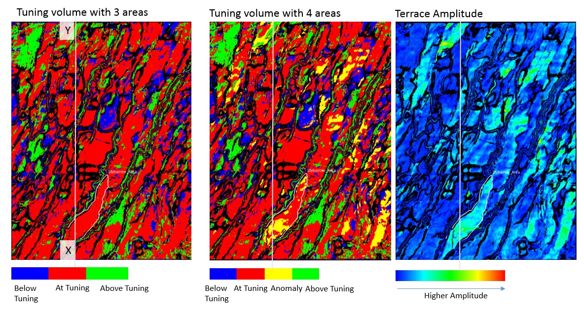
The tuning classification volume can then be data mapped on the horizon, or overlain on a slice to compare with your seismic, RGB blends or other attributes.
Above are two tuning volumes and terrace amplitude volume mapped on the same horizon. In the map with terrace amplitude, you could see that within our target reservoir area (within polygon), it shows high amplitude area where we could not differentiate the area of true amplitude and tuning amplitude. With the tuning volumes, we could tell where tuning area and anomaly area. This helps in deciding well placement in the future and avoid DHI pitfalls in amplitude.
If you want further details on the workflow, please contact us.