
High Definition Frequency Decomposition (HDFD) is one of the many unique tools and workflows available within GeoTeric. When combined with the standard frequency decomposition methods that are available, this provides the user with a powerful tool for rapidly visualising and extracting meaning from their data. As with all methods there are strengths and weaknesses of HDFD, and understanding this allows us to make the best use of these tools. In this post we will look at one approach that can give us the ability to create HDFD blends using a horizon preview, allowing us to tailor our blends while focussing on key geomorphologies.
HDFD uses a modified matching pursuit algorithm, meaning that it uses a dictionary of Gabor wavelets which are correlated to each event in the seismic data individually ( Figure 1 ). This means that the preview used for HDFD is either an inline or a crossline. Using a z slice or horizon would require processing too large a percentage of the whole survey, thus slowing the preview process. The HDFD tool provides several methods to offset this, primarily the Example Driven Interface and the Spectrogram, which allow the user to effectively interrogate the data and optimise their HDFD blend. In certain cases however it may be critical that this optimisation is done while looking at a horizon or z slice, and given some extra time this can be achieved.
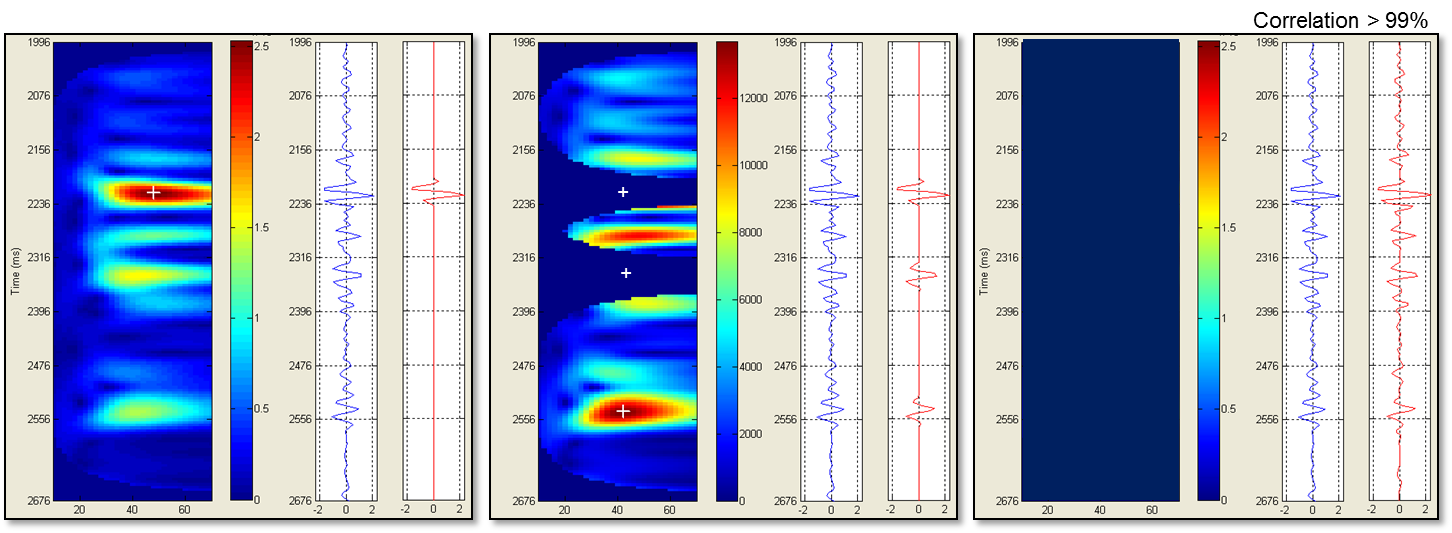
Figure 1 The HDFD algorithm in practice.
To do this we effectively separate the Frequency Decomposition from the blending. We will use the HDFD tool to produce the individual Frequency Decomposition volumes, and then use the Colour Blending tool to create the blend using a horizon preview.
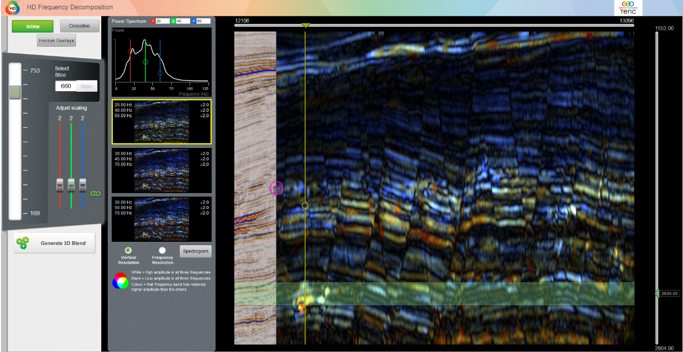
Figure 2 The HDFD tool. The three preview swatches are on the left.
The target is highlighted by the yellow line and green slab.
The target is highlighted by the yellow line and green slab.
The first step is to use the HDFD tool as normal. Using an appropriate preview line, we can analyse the feature of interest using the Example Driven Interface ( Figure 2 ). This allows us to understand the spectrum at the target level, and to compare the results of several different blends using the preview swatches. We can also move to the Spectrogram, letting us understand the frequency response at the target in a far more detailed manner. Once we have selected an appropriate blend, we can then generate these volumes as a first step, optionally unchecking the HDFD blend. Once this is complete, we can then produce a second series of HDFD volumes using frequencies offset from the original by 5 or 10Hz. If my first set of volumes used 20, 40 and 60Hz, I might then run a second set using 30, 45 and 70Hz. This can be continued as needed, until you have volumes spanning the range of useful frequencies.
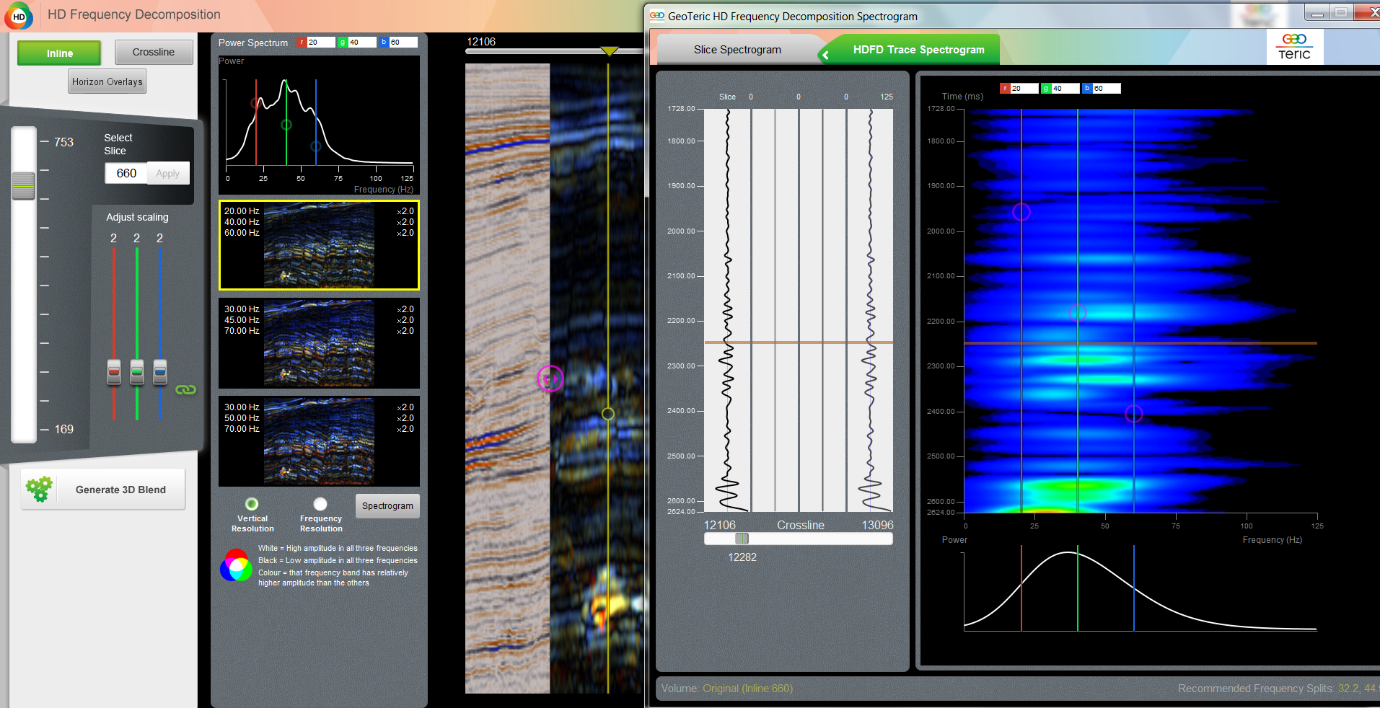
Figure 3 The HDFD tool with Spectrogram overlaid.
The yellow line shows which trace is being analysed by the Spectrogram.
The yellow line shows which trace is being analysed by the Spectrogram.
From there we can step into the Colour Blending tool. This can be found under Tools > New Colour Blend, or by clicking on the Colour Blends folder in the Project Tree. In this tool the user can blend any three volumes that they have available. This can be used to create new blends of Frequency Decomposition or edge attribute volumes. Alternatively the user could blend a mix of both, providing a blend that images both energy and structure. In this case we can use the tool to reblend our HDFD volumes while focussing on the target horizon.
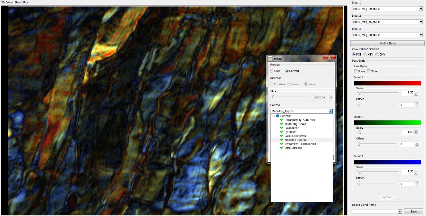
Figure 4 The Colour Blending tool. Volume selection is in the top right.
The Setup window shows the horizon selection.
The Setup window shows the horizon selection.
The HDFD volumes are selected from the drop down menus in the top right. Once we have made our initial selection, we hit the Set Blend button and from there we have the ability to select a horizon preview ( Figure 4 ). After testing different combinations of volumes, we can then manipulate the scaling factors to change the gain on the final blend. The number of volumes to choose from is obviously dependant on the amount of time spent up front, but this can be decided based on the subtlety of the target. The end result is that we have the chance to confirm that we have an optimal blend for our target, having chosen frequencies and scaling factors based on the key horizon.
This simple way of gaining new value from GeoTeric hints at the ways that the user can expand their toolbox once they have a solid understanding of the functionality available. The flexibility in GeoTeric means that new workflows are constantly being created, based only on the challenges at hand and the creativity of the user. This is just one more way that GeoTeric is Thinking About Interpretation.
