

In the previous post we covered the basics of using Geoteric’s Fault Expression tool. The aim of that post was to take the user through all of the steps required to produce a reasonable first pass product. However there are also many variations and optimisation methods that can be used to give you different options based on the data you are working with.
There are a range of different scenarios that can make detection of faults in seismic data very difficult, such as noisy data, shallow angle faults, small throws and small vertical lateral extent. It is due to this variation that there are so many potential approaches that may be worth trying for a particular scenario. In this post we will cover these variations, plus tips to guide your thinking when using Fault Expression.
Tip #1 - Understand the CMY Blend
The first step is understanding the colour blend that is used for Fault Expression. The CMY colour blend is made up of three channels: Cyan, Magenta and Yellow. Cyan is typically assigned to the Tensor attribute, which looks at changes in amplitude. Magenta is typically assigned to the Structurally Oriented (SO) Semblance attribute, which looks at changes in phase. Yellow is typically assigned to the Dip attribute, which looks at changes in the dip angle.
The CMY blend is subtractive, so when we have high values we get darker colours. If all attributes are low we get white or pale colours, and if values are high we get black or dark colours. In this way, faults are marked as dark colours in the blend.
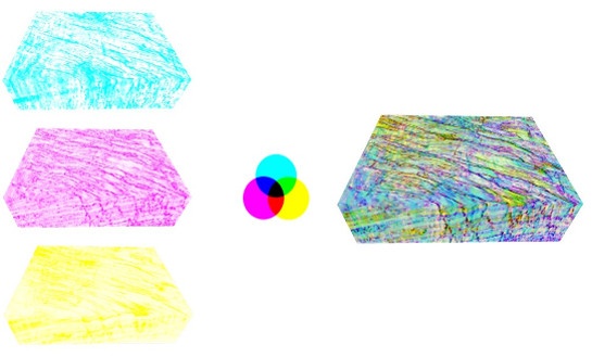
Example of the CMY colour blending process. Here we have Dip in cyan, SOSemblance in Magenta and Tensor in Yellow. In the final blend we see dark colours marking the faults.
Tip #2 - Big Faults, Big Filters
The size of our attribute windows should be relative to the size of the faults we are targeting. For exploration scale work where we are targeting large scale faults, tend towards larger windows for the attributes. This will give better continuity to the faults and less noise in the final blend. For smaller scale, intra-reservoir faults, you will need to use smaller filter sizes. This will generally result in more noise, but is more likely to identify small discontinuities. Also at this scale it is more reasonable to spend the time differentiating noise from genuine small scale faults.
Tip #3 - Fault Proportions Decide Filter Proportions
The shape of your faults should guide you in the choice of fault attribute window sizes. If you are targeting steep faults, you will generally be best off using similarly shaped windows e.g. 3 wide x 15 high. If your faults are shallower in angle, then you might move towards a wider, shorter window e.g. 9 wide x 9 high.
Tip #4 - Sharp Fault ≠ Good Fault Detect
It can be counterintuitive but we do not always need to optimise for sharp faults in the final blend. If our aim is to produce the best possible fault detect volume, this is often achieved by using filter sizes that smear the faults so as to produce a continuous fault plane. Visually we prefer sharp faults, since we can mentally connect the dots. Also, when the volume is smeared we have difficulty deciding exactly where to place the fault.
The fault detect algorithm cannot connect the dots, so it prefers a more smeared, continuous input. On the other hand, the smearing is not a problem for fault placement, since it has no trouble detecting where the peak value is.
Tip #5 - Vary Your Inputs
One of the key points in any fault workflow is that the input data is critical. This can be taken in a number of different ways. Firstly, we can decide on the optimal amount of filtering to apply before running Fault Expression. In challenging cases we will test on raw data, Noise Expression data and sometimes after filtering out noisy frequencies in Spectral Expression.
Apart from the filtering applied to the input, we can vary the input datasets themselves. In some cases we have had good results using angle stacks or azimuthal stacks to image different aspects of the faulting within a dataset. The Near stack is an obvious candidate for this, but the other options have also proved useful at times.
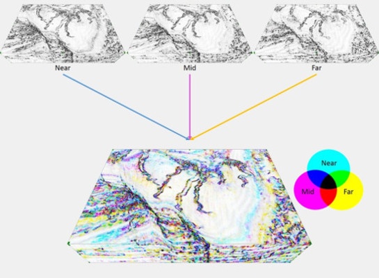
Fault Expression on angle stacks.
Edge attributes are calculated for each stack, then blended together.
Tip #6 - Fault Detect Optimisation
There are fewer options for optimising the Fault Detect algorithm, but we can still make some adjustments to improve the results. As with the attributes, we should choose the size of the Enhance Window based on the size of fault we are targeting. Once we have a choice in mind, we can also test similar options. One option is to test the current selection against a smaller enhance size combined with a higher confidence value. So if our first choice was an enhance of 3x3x6 and confidence of 3, we might test against an enhance of 2x2x4 with a confidence of 6.
Tip #7 - Fault Expression for Stratigraphy

Standard approach for parameterising Fault Expression for stratigraphic targets. Window size should be based on the size of target features.
Fault Expression can also be used to target stratigraphic features. Since the attributes are simply looking for edges in the data, it is simply a matter of tailoring them towards the edges seen in stratigraphic features. This often means using smaller windows, especially for height.
