

This will be a two-part blog post focusing on ‘Validate’, Geoteric’s Seismic Forward Modelling module that recently became available with the release of 2018.1. The tool is intended for interpreters to be able to easily test hypotheses by creating models that can be matched back to frequency decomposition results as well as reflectivity data.
This week’s post works through a simple example of testing a hypothesis using Validate. In the next post, we will go over some more advanced topics.
We begin by focusing on the Eskdale reservoir in offshore Australia’s Exmouth Basin. This field is comprised of deepwater channel sands compartmentalized by faults. We’ll be looking at the first exploration well, Eskdale-1 (Fig. 1), which found only residual oil in a 75-meter-thick sand package.
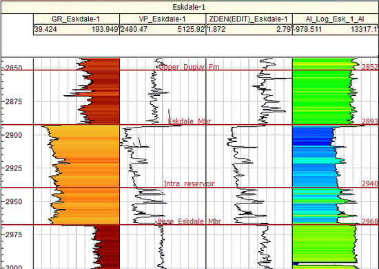
Figure 1: Gamma Ray and acoustic logs over the Eskdale reservoir in the Eskdale-1 well. Note the change in acoustic impedance at the “Intra_reservoir” marker.
Figure 2 shows a map view of the frequency decomposition RGB colour blend draped 10ms below the top of the Eskdale member. The Eskdale-2 well was drilled in a separate fault block and found economic oil, so the task of defining the reservoir extents both in terms of reservoir quality sand and fluid content becomes critical if the field is to continue to be appraised and developed. As evidenced by the map below, GeoTeric’s Frequency Decomposition attributes reveal many aspects of the depositional system. But the question has always been, “what do the colours mean?”. Validate can help answer that question.
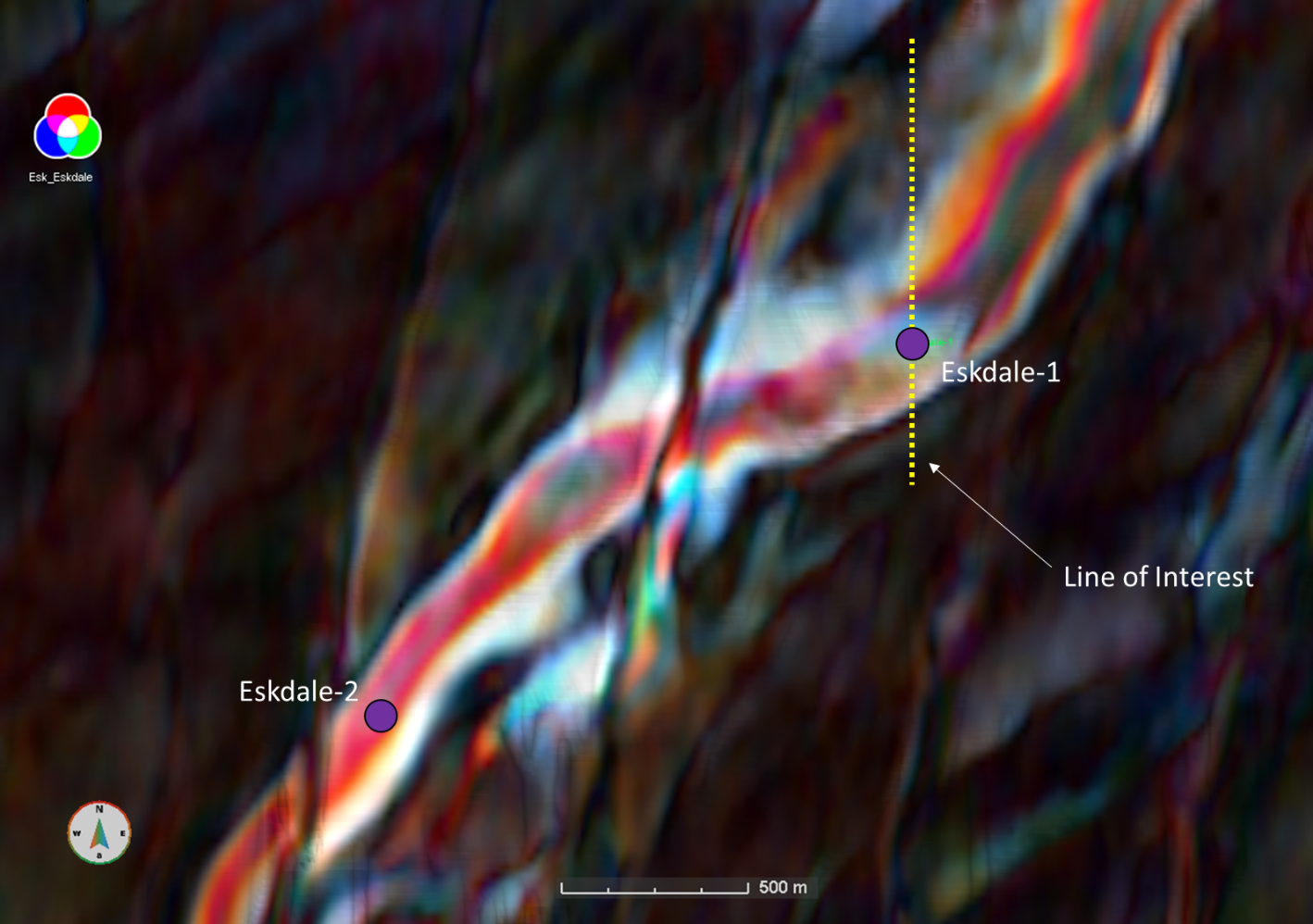
Figure 2: Uniform Constant Q Frequency Decomposition RGB colour blend (18-35-57Hz) showing Eskdale channel. The blend is draped 10ms below the top of the Eskdale member. The yellow dotted line represents the Validate cross-section.
In this example, we'll use Validate to help refine the geological model to gain a better understanding of the depositional makeup of the channel. In the map above we can see the channel clearly but, upon close inspection, several questions are left unanswered. What does the variability of the colours along the channel axis mean? What do the white to grey-blue colours north of the Eskdale-1 well represent; levee, crevasse splay, a single event or multiple events? Where are the sand boundaries? To answer these questions, we've set up a Validate session where we have tested three hypotheses using a cross-section through the well (shown in Figure 2). The layer boundaries were created through a combination of horizons and freehand drawing layer boundaries.
Looking at the seismic reflectivity data shown in Figure 3a, we see that the Eskdale-1 well penetrated the main channel body at it’s thickest point. Note the ‘tail’ that continues out to the right of the main channel body. Do these features together represent a continuous, homogeneous depositional element or could the ‘tail’ be a separate feature such as a crevasse splay? Model 1, Figure 3b, shows the first iteration of modelling where we model this feature as one homogeneous unit using well log properties from the entire Eskdale interval. This is the initial model that we will continue to modify as we gain new insights. The dark green interval represents a shale sequence that was eroded into by the channel while the lighter green represents the over/underburden. Rock properties for these sequences are also taken from the Eskdale-1 well.
Both the modelled reflectivity and FD show little correlation to the actual seismic. The ‘tail’ in the synthetic reflectivity does not show the drop in amplitude contained in the real data and it’s too bright in the synthetic FD. We can conclude that the features in question are likely not one singular depositional event.
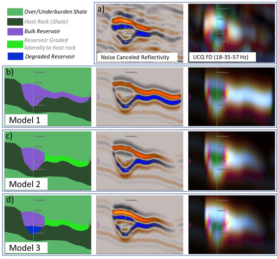
Figure 3: Reservoir models and their synthetic responses in both reflectivity and FD space. a) Actual data – noise cancelled reflectivity and RGB colour blend sections through the line of interest shown in Fig.2. b) Model 1: channel and ‘tail’ represented as one homogeneous package. c) Model 2: ‘tail’ grades from sand on the left to shale on the right. d) Model 3: diagenetic degraded reservoir is added at the base of the channel.
Moving to Model 2, shown in Figure 3c, we've now separated the ‘tail’ into its own unit and modelled it as a sand grading to shale from left to right. In this case, we are treating this event as a possible crevasse splay, where reservoir quality gradually decreases with distance. In the modelled reflectivity we can now see that the drop in amplitude matches better with the real data and the frequency decomposition moving from white-yellow to dull grey-blue from left to right also has a better match.
So now we think we've figured out what the ‘tail’ might be, but we still don’t have a good match in the main channel body. Both the seismic and FD seem to be showing more variability than my models are capturing. Looking back at Figure 1, we see that there is a transition in the calculated AI log at about 2940m. we've marked this as “Intra_reservoir” on the log section. Core plug data taken in this interval suggests that diagenesis has taken place in this basal unit. Altered cement in this interval could lead to poorer reservoir quality and may explain the higher values observed in the AI log. Given this, we've segmented the reservoir in Model 3 (Fig. 3d) into an upper high-quality sand unit and a lower poor-quality sand unit. We can see that now my amplitudes along the entire channel body match much better in the synthetic reflectivity, and we've matching the internal channel events much better as well. Comparing the FD in Model 2 and 3, Note that both models accurately capture the colour patterns at the channel edges – bright red/magenta into bright orange/yellow/white – but Model 3 does a much better job capturing the colour pattern along the well in the thick part of the channel.
After this brief modelling study, we've been able to make several new insights about the FD colour blend and the geology it represents:
• The ‘tail’ seen in the seismic and represented in the FD map view as the light blue-grey features north of the Eskdale-1 well is likely a crevasse splay or levee deposit.
• Channel edges are represented in the FD as distinct red/magenta to yellow/orange/white lineations.
• The internal variability seen in the main channel in the FD is caused, at least in part, by the vertical juxtaposition of a higher quality reservoir sand overlaying a degraded reservoir sand.
Armed with these new insights, we now have less uncertainty in the depositional model and we can use the FD colour blend to create a visual representation of that it so we can communicate the understanding to colleagues and management. This can be used to influence critical decisions like whether to appraise the field and where to place appraisal wells.
For further work, we could perform a fluid substitution to see the change in the model using an oil wet reservoir (see next week’s post!) and we could populate a depositional model semi-automatically using Geoteric’s Interactive Facies Classification module.
