

This is the second part of a two-part (part 1) blog post focusing on ‘Validate’, Geoteric’s seismic forward modelling module that recently became available with the release of 2018.1. The tool is meant for interpreters to be able to easily test hypotheses by creating models that can be matched back to frequency decomposition results as well as reflectivity data.
Last week’s post works through a simple example of testing a depositional hypothesis using Validate. This week, we'll go through a fluid substitution example and discuss the impact of using “ALL” vs. “AVERAGE” rock properties on modelling results.
Fluid Substitution
We'll focus now on the Stybarrow field, a slightly shallower turbidite reservoir just north of the Eskdale well used in last week’s blog. The Stybarrow-1 well discovered an 18 meter thick oil bearing sand called the Macedon formation (Fig. 1). The well penetrated the high amplitude portion of the Macedon reflector which dims downdip as it truncates against a fault. We'll use Validate to investigate the nature of this dimming. Is it due to shaling out or perhaps an unresolved fluid contact?

Figure 1: Model 1, reservoir properties at the well are carried throughout the reservoir (red unit).
In the following set of figures (Figs. 1, 2, and 3) we’ve created an earth model with separate upper and lower shale layers, the green layers, encompassing the red Macedon reservoir unit. In each of the three scenarios, we modify only the reservoir in the down-dip region. A 33Hz Ricker wavelet is used in the synthetic reflectivity and the frequency decomposition in both the real and synthetic colour blend is a 30-40-60Hz Uniform Constant Q Frequency Decomposition.
Figure 1 shows a case where the reservoir properties remain constant throughout. We see a good match at the well in both the synthetic reflectivity and colour blend, but the downdip portion does not capture the dimming that’s seen in each.
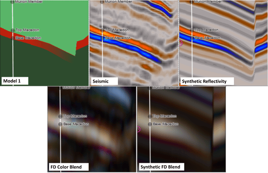
Figure 2: Model 2, reservoir properties from the well are transitioned down-dip into the underburden shale properties.
In Figure 2, we ‘transition’ the down-dip portion into shale, as shown in the upper left panel. In this case, we do see dimming in the down-dip region of the synthetic reflectivity but the response is perhaps too dim. The dimming is present in the synthetic blend as well, but the colours are not matching well. The frequency decompositon blend on the left goes from magenta to white to orange/yellow from bottom to top while the synthetic only goes from a dimmer magenta into a grey/blue.
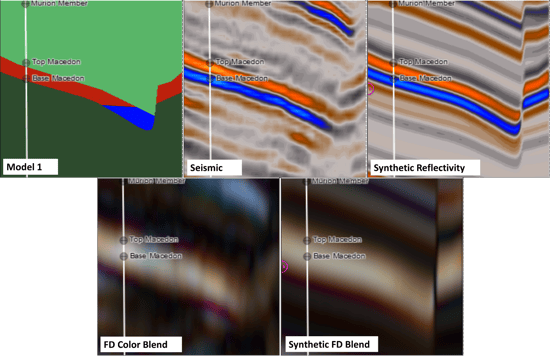
Figure 3: Model 3, a down-dip water leg is added to the reservoir using fluid substitution.
Moving to Model 3, shown in Figure 3, we've modified the model to simulate the effect a down-dip water leg would have on the seismic. To do this, we set up the fluid substitution shown in Figure 4. This is a snapshot of Validate’s ‘Rock Properties Manager’ where we’ve created a new rock under the ‘Fluid Substituted Rocks’ tab. Inputting my Vp, Vs, and density logs along with porosity, shale volume, and water saturation logs we're able to calculate the fluid subbed response using a modified Gassmann calculation after Simm, 2007. We can adjust or accept the default fluid properties at the bottom of the window in Figure 4 and use the slider bar to substitute for any water/oil or gas/oil mixture we choose. In this case, we’ve simply replaced the oil with 100% brine. This has the effect of slightly increasing both compressional velocity as well as bulk density (see green well logs, denoting fluid subbed portions of the logs in Figure 4). The synthetic reflectivity at the top right of Figure 3 now shows a closer match to the dimming seen in the actual seismic. The dimming in the synthetic frequency decomposition now also matches better and the colours, while not a perfect match. They now follow the magenta to white to orange base-to-top sequence described above more closely.
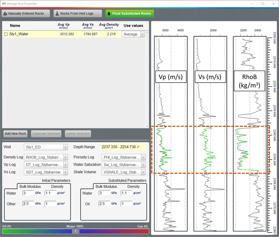
Figure 4: Fluid substitution pane within Validate’s Rock Properties Manager. Note green log portions showing depth interval over which the calculation is taking place and the fluid subbed values. The slider bar at the bottom can be used to easily change the oil/water or gas/water mixture at any time.
Now that we’ve shown the potential for, and possible position of, a down-dip water contact in the reservoir we can calculate attributes or perform inversions to help better delineate the location of the contact, calculate STOIIP, work with a rock properties or QI practitioner to perform more in-depth modelling, and ultimately make decisions on where to place appraisal wells.
Rock Properties in Validate: ‘All’ vs. ‘Average’
In the Rock Properties Manager tab in Validate, the user has the choice between “ALL” or “AVERAGE” in the ‘Use values’ column (see Fig. 4 above) for both rocks from well logs and fluid substituted rocks. If the latter is chosen, the layer that rock is assigned to will use the harmonic mean of the log properties from the selected depth interval as a single value throughout. If the former is chosen, the well log properties from the selected depth interval will be isoproportionally propagated throughout the layer assigned to that rock. Why would we use one over the other? Are there specific situations when one is more appropriate than the other? Let’s take a look.
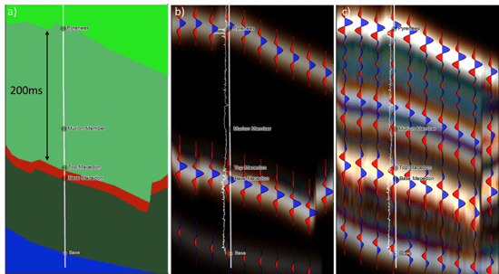
Figure 5: a) Model geometry. Properties from well are used as layer properties. b) AVERAGE rock properties synthetic blend with acoustic impedance log. c) ALL properties blend with acoustic impedance log.
Figure 5a shows a zoom out of the model used in the fluid sub example above. Figures 5b and 5c show two corresponding synthetic colour blends with the synthetic reflectivity overlaid in wiggle trace. In Figure 5b we’ve used ‘AVERAGE’ values for each layer in the model, while Figure 5c shows the result when ‘ALL’ values are used. Comparing these two panels, several observations can be made:
- The ‘ALL’ model has a much wider range of colours and is more detailed in both the frequency decomposition and reflectivity.
- The ‘ALL’ frequency decomposition synthetic is much brighter than the ‘AVERAGE’ one.
- The Macedon unit (red layer in Fig. 5a) is a trough-to-peak pair using ‘ALL’ properties but it appears to become a near zero-phase peak when the ‘AVERAGE’ properties are used.
Why should there be such a striking difference between the two models? The answer, in part, can be gleaned from the diagrams shown in Figures 6 (taken from Partyka, et al., 1999) and 7, which demonstrate the importance of thin beds in relation to spectral decomposition. Figure 6 shows an input source wavelet in both the time and frequency domains, a cartoon of a thin bed and the travel paths of the reflections from the top and base of the bed, and the resulting thin bed reflection in both the time and frequency domains. This diagram is similar to the setup of our model; the thin bed being our Macedon unit and the overburden being our thick green unit. Note the notches in the amplitude spectrum of the reflected wavelet.
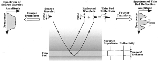
Figure 6: Source wavelet amplitude spectrum compared to the filtered spectrum resulting from interfering top and base reflections off a thin bed. From Partyka, et al., 1999
This relates to our example because when using ‘AVERAGE’ properties in thick layers as in Fig. 5b, we are removing variability from the model. By doing this, we are effectively whitening the spectrum by removing or reducing notches (Fig. 7). The result is a frequency decomposition model with little variation and a poor match to the frequency decomposition derived from the seismic. Conversely, using ‘ALL’ properties for the thicker layers introduces more variability – more thin beds of various temporal thicknesses result in more interference. This explains our observations that the model using ‘AVERAGE’ properties is both dimmer and less colourful than the one using ‘ALL’ properties.
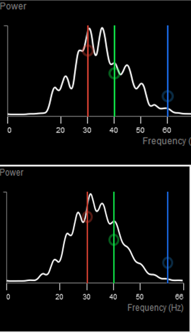
Figure 7: Amplitude spectrum of the ‘ALL’ model (above) and the ‘AVERAGE’ model (below). Note the wider bandwidth, deeper notches, and higher magnitudes in the upper frequency range for the ‘ALL’ model.
The character of the Macedon reflection is easily explained as well and similarly has to do with averaging over large intervals. We noted above that the reflection appears to have a phase rotation when using the ‘AVERAGE’ properties, but this is not the case. Upon closer inspection, we see that the leading trough is still present but is very weak. Averaging over the large green interval above the Macedon in Figure 5a has led to a lower acoustic impedance layer above the sand that is represented in the ‘ALL’ model. Since the impedance value is closer to that of the sand, a lower reflection coefficient at the top of the sand results in a much weaker reflection – and a poor match to the seismic.
At this point, we’ve demonstrated that in this particular case it is more prudent to use ‘ALL’ well properties to populate the model. But there are many situations when using ‘AVERAGE’ properties is completely justifiable. Indeed, experienced practitioners in any geological modelling application would counsel starting simple and add complexity as needed, so using average properties at least, to begin with, would certainly be advisable in many cases. It’s worth noting that the model in Part 1 of this blog post from last week used entirely ‘AVERAGE’ well properties and returned an optimal result in both reflectivity and RGB space. The reason for this is that the Eskdale model was composed entirely of thin beds, so changing between ‘ALL’ and ‘AVERAGE’ properties has little effect on reflectivity and interference.
In practice, the decision whether or not to use ‘ALL’ or ‘AVERAGE’ rock properties depends upon the size and scope of the model and the properties of the geology in question. Luckily, Validate makes it very easy to switch back and forth between the two so that the accuracy of either method can be tested. This practice is almost always advisable.
We'll close with some rules of thumb to consider when working through a Validate session. These are meant as general guidelines and will not necessarily be applicable to all situations. Caution should always be taken to make sure any modelling decisions are fit for purpose and make sense for the geology and seismic in question. Note also that in some cases of sparse or inconsistent well data, it may become necessary to use neither, and come up with sensible values to be entered as manual rock properties.
When to use ‘AVERAGE’ properties:
- At the start of a workflow, especially when setting up the model and checking polarity.
- When geometry precludes using ‘ALL’ properties:
- Model interval is significantly thicker or thinner than well interval. This will result in the model properties being stretched or squeezed, respectively, relative to their actual temporal thickness.
- Layers being modelled have irregular geometries or lateral terminations that do not lend themselves well to isoproportional property layering
- When transitioning layer properties.
When to use ‘ALL’ properties:
- When the model calls for more vertical geologic variability than captured in the drawn layer model. This can be especially significant when trying to match the synthetic RGB colour blend.
- When averaging over intervals results in erroneous properties. Pay close attention to this especially in AVO class 2 environments (sand impedance is near shale impedance).
References
Partyka, G., Gridley, J. and Lopez, J. [1999]. Interpretational applications of spectral decomposition in reservoir characterization. The Leading Edge, 18 (3), 353-360.
Simm, R. [1999]. Practical Gassmann fluid substitution in sand/shale sequences. First Break, 25, 61-68.
Suggestions for Further Reading
Han, C. [2018]. Understanding frequency decomposition colour blends using forward modelling – an example from the Scarborough gas field. First Break,36,53-60
Cooke, N., Szafian, P., Gruenwald, P. and Schuler, L. [2014]. Forward modelling to understand colour responses in an HDFD RGB blend around a gas discovery. First Break, 32, 87-93.
Widess, M.B. [1973]. How thin is a thin bed? Geophysics, 38, 1176-1180.
