

Part 2 - Peak Frequency by Magnitude
In Part 2 of this blog post, adding the amplitude of the Magnitude volume to Peak Frequency volumes helps with understanding the thickness and lithology variations within the data.
The next step is to create a volume where hue will correspond to frequency and saturation of the colour corresponds to its amplitude in the Magnitude volume.
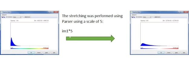
Figure 1: Results of stretching discrete frequency volumes
Depending on the amplitude distribution in the discrete frequency volumes it may be useful to perform stretching to achieve maximum coverage of the colour map. Each of the discrete frequency volumes will need to be rescaled, to fit the numerical range of each volume into its associated colour bin, created in the previous blog. It is recommended to use uniform stretch if the input volume was spectrally balanced, and max stretch if original volume is used.
This will be illustrated on the example: for the volume corresponding to 20 Hz the range, its values should correspond to the interval 1345-2016 on the colour map created; 26.67 Hz to 2017-2672; and so on for all intervals according to Table 1.
To perform this operation a batch job is created in the Batch and Processing Framework using the following formula for each volume:
lowerlimit*(1-(im1/32767))+upperlimit*(im1/32767)
lowerlimit correspond to the minimal value of the frequency range (Table 1); upperlimit – maximum value for the interval frequency range (Table 1); im1– scaled discrete frequency magnitude volume; 32767 – maximum value for the im1 (16 bit in this case, if using 32 bit data the value will be 2147483648).
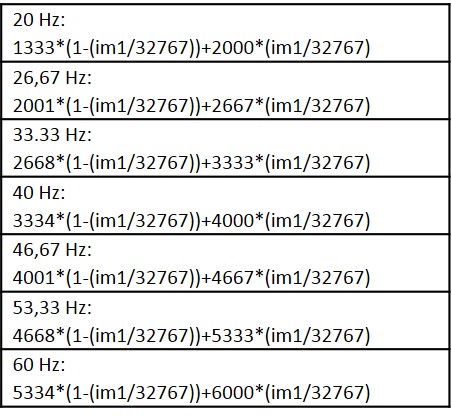 |
Table 1 |
After running this step, 7 volumes will be created and added to Project Tree.
The next step is to combine those volumes with the Peak Frequency volume, where in each frequency bin, the saturation varies according to amplitude of the discrete frequency volume. The following equation should be used in Parser:
(im1=2000)*im2+(im1=2667)*im3+(im1=3333)*im4+(im1=4000)*im5+(im1=4667)*im6+(im1=5333)*im7+(im1=6000)*im8
Here im1 – PeakFrequency volume; im2…im8 – corresponding discrete frequency volumes.
After this volume is generated and added to Project Tree the volume can be visualised with the corresponding histogram. As can be seen in Table 4, the Envelope, creates a bright spot at the center of field, which is related to tuning. In the resultant Peak Frequency volume with the Magnitude data included, this area is no longer a bright spot and is on the medium to high frequency range and therefore could be considered not the best reservoir quality.
Using Discrete Frequency volumes on small sections of the data could be very useful in helping to determine lithology variations and add information to the RGB Blend, to help de-risk potential drilling locations.

Figure 2: From left to right - Envelope, Peak Frequency and Peak Frequency with Magnitude
(By Pavel Jilinski)
