

Tracking and Fill Modes
Geoteric’s Adaptive Horizons have a variety of tracking and fill modes to allow the interpreter to extract a horizons surface in a fast and accurate way, while being cognitively intuitive. Geoteric’s tracking modes are interactive as all the possible routes through the data are determined using Graph Theory, and can be previewed in both the 3D viewer and in the 2D Interpretation window. The Fill modes can be easily chosen in the Base Map window or in the 3D window if tracking on a probe.
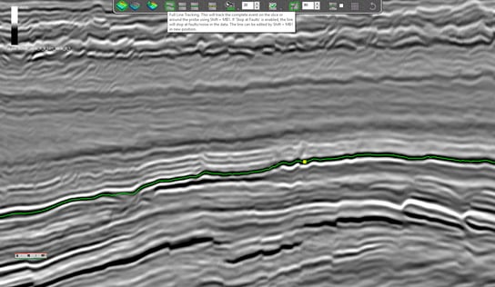
![]() Tracking Modes: Full Line Tracking: this will utilize Graph Theory to find the best possible interpretation across the entire line. This option is useful when interpreting regional events that are laterally continuous and not heavily faulted. If “Stop at Faults” is enabled, the line will stop at discontinuities and faults, allowing the interpreter to make the cross fault interpretation.
Tracking Modes: Full Line Tracking: this will utilize Graph Theory to find the best possible interpretation across the entire line. This option is useful when interpreting regional events that are laterally continuous and not heavily faulted. If “Stop at Faults” is enabled, the line will stop at discontinuities and faults, allowing the interpreter to make the cross fault interpretation.
 |
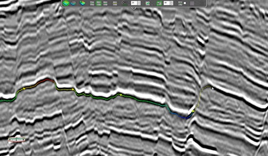
![]() Piecewise Tracking: allows the user to pick points along a reflector, the tracker will find the best path between points along the horizon (also using Graph Theory). A preview of the line is available interactively as the mouse is moved to aide with the interpretation. The preview line ensures that picks are only placed where they are needed thus reducing the amount of clicking required to complete your interpretation.
Piecewise Tracking: allows the user to pick points along a reflector, the tracker will find the best path between points along the horizon (also using Graph Theory). A preview of the line is available interactively as the mouse is moved to aide with the interpretation. The preview line ensures that picks are only placed where they are needed thus reducing the amount of clicking required to complete your interpretation.
 |
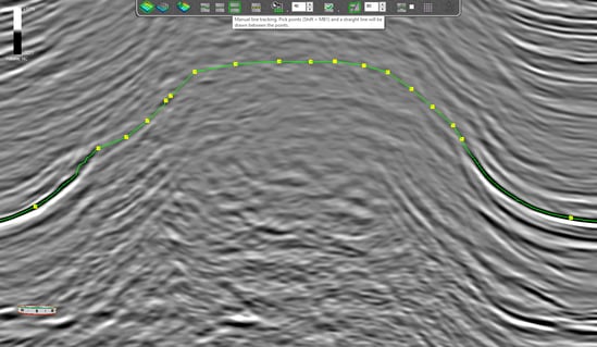
![]() Manual Line Tracking: This is helpful when the data quality is very poor and the interpreter would like to force an interpretation through, for example through salt diapirs such as below:
Manual Line Tracking: This is helpful when the data quality is very poor and the interpreter would like to force an interpretation through, for example through salt diapirs such as below:
 |
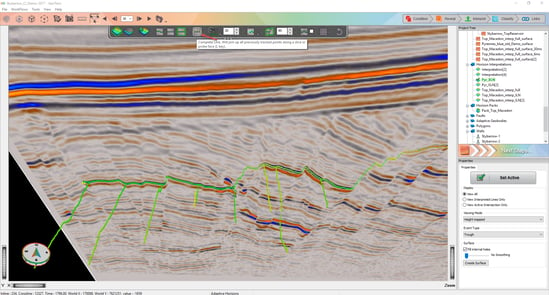
![]() Complete Line: this option will join up previously tracked points along a slice. This is useful to create a grid of the interpretation if the horizon has been interpreted in one direction. Enabling the horizon to be quickly QC’d and completed saving time and aiding efficiency whilst maintaining the accuracy of the interpretation.
Complete Line: this option will join up previously tracked points along a slice. This is useful to create a grid of the interpretation if the horizon has been interpreted in one direction. Enabling the horizon to be quickly QC’d and completed saving time and aiding efficiency whilst maintaining the accuracy of the interpretation.
 |
Fill Modes:
The fill modes auto-track the data always honouring any interpreted lines and is constrained laterally either by the extent of the probe or the defined area on the base map.
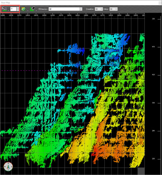
![]() Waveform: Correlates the waveform of each point along all interpreted/accepted lines to guide the tracking over the selected area on the base map or the probe. The acceptance level controls how close the tracked area needs to be to the seed points, the lower the acceptance level, the closer to the input, the higher the acceptance level, the more room for growth. This method, is the fastest and is best suited for regular seismic data. The waveform of each point is treated individually, so if the character of the horizon changes laterally the horizon adapts to this change.
Waveform: Correlates the waveform of each point along all interpreted/accepted lines to guide the tracking over the selected area on the base map or the probe. The acceptance level controls how close the tracked area needs to be to the seed points, the lower the acceptance level, the closer to the input, the higher the acceptance level, the more room for growth. This method, is the fastest and is best suited for regular seismic data. The waveform of each point is treated individually, so if the character of the horizon changes laterally the horizon adapts to this change.
 |
![]() Amplitude: Correlates the amplitude of each point along all interpreted/accepted lines to guide the tracking over the selected area on the base map or the probe. The acceptance level controls how close the tracked area needs to be to the seed points.
Amplitude: Correlates the amplitude of each point along all interpreted/accepted lines to guide the tracking over the selected area on the base map or the probe. The acceptance level controls how close the tracked area needs to be to the seed points.
![]() PDF: Calculates a Probability Density Function (PDF) of the interpreted/accepted seeds and uses this to guide the tracking. The acceptance level controls the PDF and how much of its data is used to track. When tracking on the HSV blend, all 3 volumes of the blend are used as inputs, so the PDF option is the only way to capture this information, and is therefore the only choice available when tracking on a blend.
PDF: Calculates a Probability Density Function (PDF) of the interpreted/accepted seeds and uses this to guide the tracking. The acceptance level controls the PDF and how much of its data is used to track. When tracking on the HSV blend, all 3 volumes of the blend are used as inputs, so the PDF option is the only way to capture this information, and is therefore the only choice available when tracking on a blend.
![]() Graph Theory: Calculates the optimum surface that intersects with the interpreted/accepted seed points using graph theory. This option fills the area selected completely, without leaving any holes, however it is also the most computationally intensive, so it is recommended to select smaller grid areas to fill.
Graph Theory: Calculates the optimum surface that intersects with the interpreted/accepted seed points using graph theory. This option fills the area selected completely, without leaving any holes, however it is also the most computationally intensive, so it is recommended to select smaller grid areas to fill.
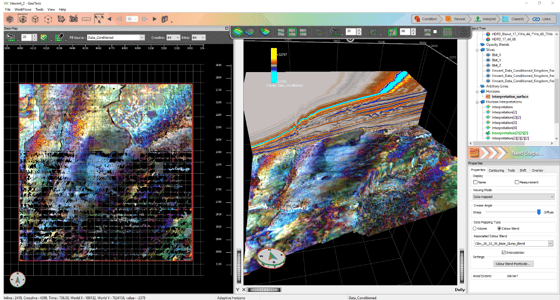
In the example below, a potential base slump event was filled using the waveform option and has a Frequency Decomposition RGB blend mapped prior to the surface generation, therefore giving the interpreter a better understanding of the geology throughout the interpretation process.
Part 3 provides more details on the 3D surface editing option.
