
GeoTeric's Adaptive Fault workflow has been developed to produce rapid and accurate fault interpretations. This workflow makes use of GeoTeric's Noise Expression to produce the cleanest possible input data, Fault Expression to capture all fault information in one blend, and Adaptive Faults to provide the most intuitive fault interpretation experience. One tool that can add extra value at the end of this workflow is the Interactive Fault Slicing, which allows rapid comparison of responses across a fault plane.
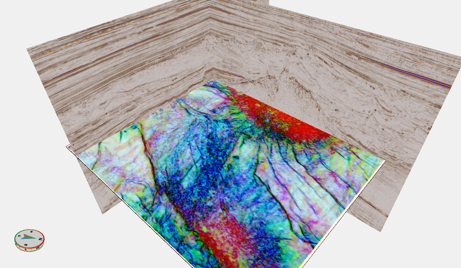
Figure 1: Fault Interpretation set up with a slice consisting of a CMY Blend, and ILN and XLN slices consisting of Conditioned seismic data.
We begin by first creating the required fault plane. In the above scene, Figure 1, we see the standard set up for fault interpretation in GeoTeric, consisting of the Conditioned Ceismic on the ILN and XLN slices, and the Fault Expression CMY Blend on the slice. Displaying the CMY Blend on the slice allows the detailed fault attribute information in the CMY Blend to guide and tie together the interpretation from the seismic. Fault interpretation in GeoTeric can be done on both colour blends and volumes and all three slices. Given the amount of information in the CMY Blend, it can greatly speed up interpretation in challenging areas.
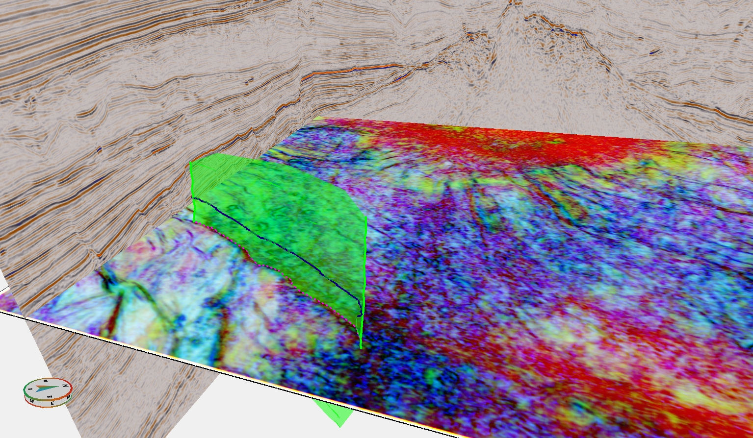
Figure 2: This fault was interpreted with only 3 sticks, one on the slice and 2 on the ILN slice. The data following ability of the Fault Plane, increases the accuracies with fewer fault sticks.
Once we have decided which fault to interpret, we can begin by interpreting a horizontal fault stick along the slice of the CMY Blend. Vertical fault sticks can then be interpreted on the ILN and/or XLN slices at the edges of the fault. The fault sticks are data following, each fault stick will snap to discontinuities in the volume or blend being interpreted. Once we have multiple fault sticks, the fault surface generation can be set to data following, giving the results seen in Figure 2, using only two vertical sticks and one horizontal stick.
- To create the Fault Surface right-click on the Fault Set in the Project Tree and select 'Create Surface'.
- Next visualise the Fault Surface in the 3D Scene.
- In the Properties panel for the Fault Surface, select 'Data Mapped' from the 'Viewing Mode' dropdown. See Figure 3.
- Select Colour Blend and choose an 'Associated Colour Blend' from that dropdown.
- Next go to the 'Interactive Fault Slicing' tab, and check the 'Enable Fault Translation' box.
Once we have enabled the Fault Slicing, the Fault Surface can be moved in 3D (lateral and vertical movement) or 2D along the XY plane (does not move vertically). We can move the plane by either typing in the boxes, or dragging the green arrow. Finally, we can duplicate the fault, using the 'Save as New Fault' button to compare the responses on the original fault surface to the moved fault surface.
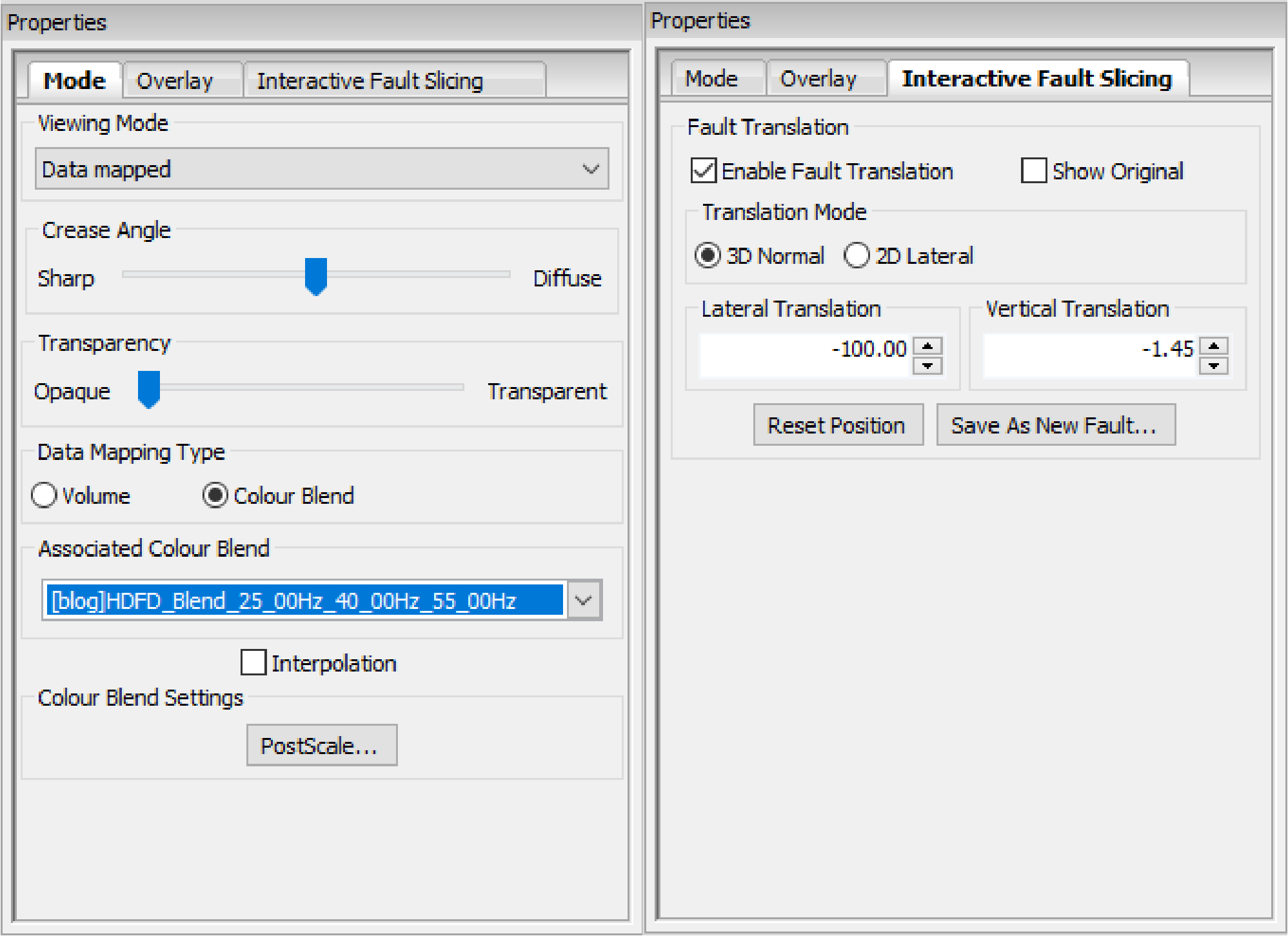
Figure 3: Fault Surface Properties Menu to display the RGB Blend and activating the Interactive Fault Slicing.
The Fault Slicing tool can be used to effectively compare the response across the fault plane, Figure 4. This can be used with the High Definition Frequency Decomposition to compare subtle changes in the frequency and amplitude characterstics, the CMY to compare changes in continuity, or to collect the information required to build Allan diagrams.
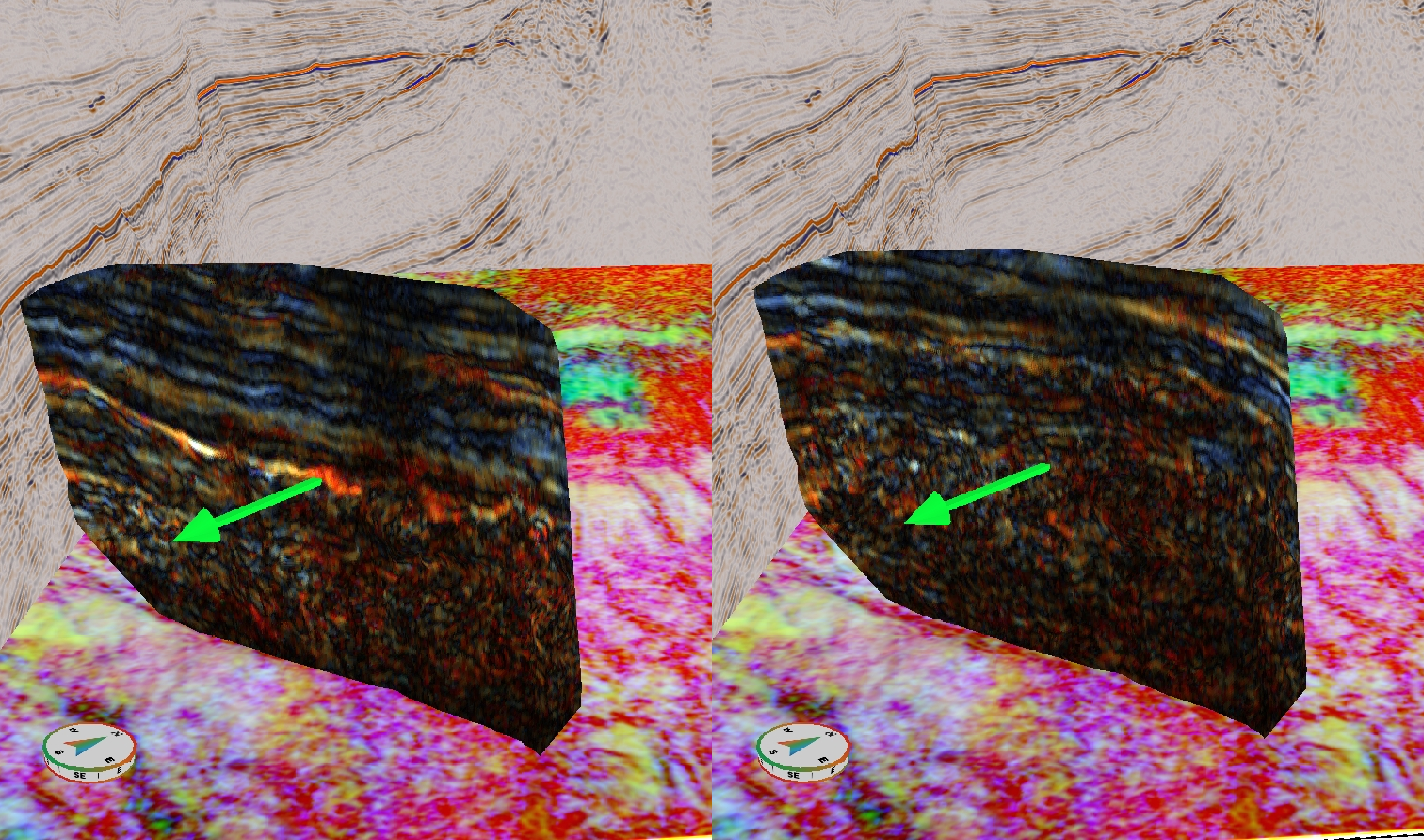
Figure 4: Fault Surface with the RGB Blend displayed, and the arrow to move the slice, left. On the right the fault slice is moved to compare the RGB response on the other side of the fault.
