
GeoTeric can be used very effectively in a multi-volume environment to screen for differences in AVO, 4D or Multi-Azimuth responses. In some cases, the reflectors are not well aligned between the stacks that we are comparing or there is an unexpected frequency change between the stacks, so any interpretation on those areas might be unreliable.
Misalignment of stacks can cause false positive AVO anomalies or false 4D/Multi-Azimuth interpretations, so being able to highlight those unreliable areas can help to increase the confidence on the multi-volume analysis.
This advanced workflow involves the use of the Parser in order to highlight areas of misalignment or frequency changes. The
Parser can be found under Processes & Workflows > Processes > Volume Maths > Parser.
Phase alignment: “peaks volume” and “troughs volume”
To start our phase alignment analysis, we can just bring the two volumes we are interested to compare into the Parser, and type the Parser expression (im1>0)*im2. This will generate a “peaks volume” where the peaks of the 1st input volume will be replaced by whatever data we have in the 2nd volume. So if we see any troughs in the resulting volume, it means that the alignment is poor in those areas.
Similarly we can apply (im1<0)*im2, and that will give us a “troughs volume” where any positive values will indicate areas of poor alignment.
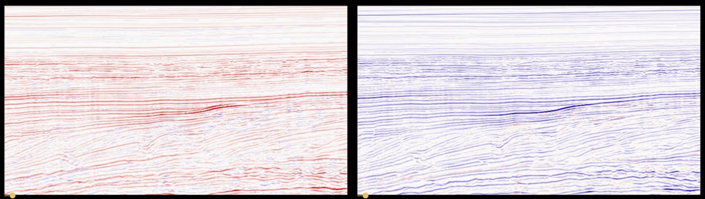
“Peaks volume” (left) and “troughs volume” (right) showing a fairly good stack alignment
Phase alignment: Bedform stack
A much more detailed QC can be achieved by using a Bedform stack. We can compute the Bedform indicator attribute for each of the stacks, and then combine the Bedform attributes using a parser expression. The example below is a combination of three angle stacks, but a similar approach can be followed for other volumes. The Parser expressions we need to use are:
For 32bit:
((((im1>700000000)*im1)+((im1<-700000000)*im1))+(((im2>700000000)*im2)+((im2<-700000000)*im2))+(((im3>700000000)*im3)+((im3<-700000000)*im3)))/3
For 16bit:
((((im1>10000)*im1)+((im1<-10000)*im1))+(((im2>10000)*im2)+((im2<-10000)*im2))+(((im3>10000)*im3)+((im3<-10000)*im3)))/3
For 8bit:
((((im1>170)*im1)+((im1<90)*im1))+(((im2>170)*im2)+((im2<90)*im2))+(((im3>170)*im3)+((im3<90)*im3)))/3
These Parser expressions are simply (im1+im2+im3)/3, but as we want to remove the doublet values in each of the Bedform attributes they become a bit more complex.
If the output is displayed using the Azimuthcolour map, areas with good alignment will be seen in black, areas with dispersion along a peak in red, and areas with dispersion along a trough in blue. The lighter the blue and red colours, the worse the alignment.
If the output is displayed using the Azimuthcolour map, areas with good alignment will be seen in black, areas with dispersion along a peak in red, and areas with dispersion along a trough in blue. The lighter the blue and red colours, the worse the alignment.
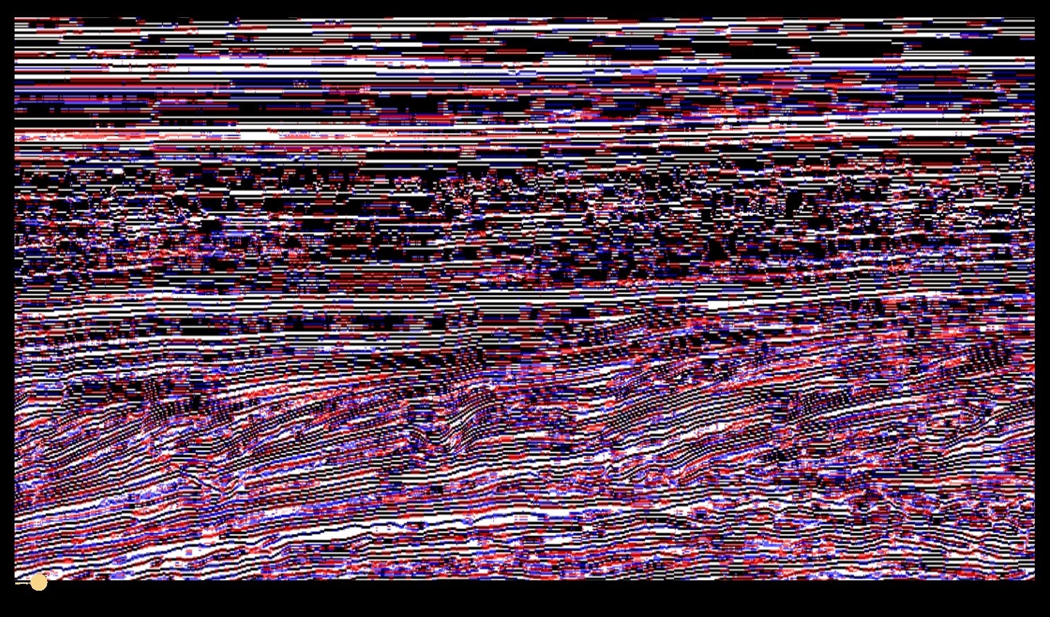
Bedform stack volume showing areas with good alignment in black and areas of worse alignment in red and blue.
Frequency change QC
The frequency changes across our stacks can be QCed by comparing the instantaneous frequency attributes. The first step involves computing the Instantaneous Frequency attribute for two of the volumes (such as near and far), then applying a Smoothing (can be found under Processes & Workflows > Processes > Attributes > Structural attributes) using a median option and a 3x3x5 footprint to each of the Instantaneous Frequency volumes. Then the Frequency QC volume can be produced using the following Parser expression:
ABS(((im1>0)&(im2>0))*(im2-im1))
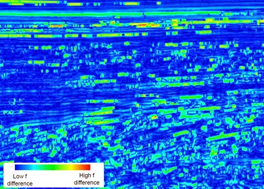
Frequency change QC volume showing minor frequency differences between two stacks.
In summary, by applying this multi-volume similarity workflow, we can identify areas of misalignment in our stacks and increase our confidence in any further AVO, 4D or Multi-Azimuth analysis.
