

This is the last part of our series on AVO screening in Geoteric.
Scaled reflectivity is a volume that results from a rotation of the gradient-intercept crossplot using a certain χ angle. If the right χ angle is used, it will highlight fluid effects. We covered how to create the Gradient and Intercept volumes in part 3. The scaled reflectivity can be calculated using the following formula (Whitcombe et al., 2002)
Rs= R(0)cosχ +Gsinχ
Which is the following equation using Geoteric’s Parser:
im1*cos(χ*pi/180)+im2*sin(χ *pi/180)
Where im1=intercept and im2=gradient
Estimating the χ angle
While estimating the optimum χ angle is a task that normally involves well calibration and seismic inversion, an approximation can be achieved by estimating the angle of the dominant trend from the Gradient-Intercept crossplot and consider that angle to be the lithology trend. Our optimum χ angle is then the angle of that trend plus 90°, as we can assume that the fluid trend is orthogonal to the lithology trend.
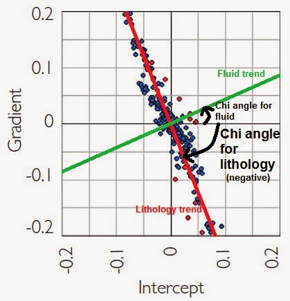
Calculating the χ angle using this approach is again a source of uncertainty as many assumptions are made.
One way of doing this angle estimation without requiring access to a cross plotting tool, is to create a Gradient divided by Intercept volume and look for the most common value on the histogram. We can use the following Parser expression to calculate the G/I volume:
Parser= (im1/im2)*scale
Where im1=gradient and im2=intercept. The scale factor is required to keep the resolution on the output volume, as only integer values are supported. For instance for 16bit data a scale factor of 1000 is usually enough. For 32 bit we have used 100000000.
If we look at the histogram of this volume, we can read the most common value of the histogram, divide it by the scale factor that we used and calculate the arctan of that value. The χ angle is 90° plus our calculated angle.
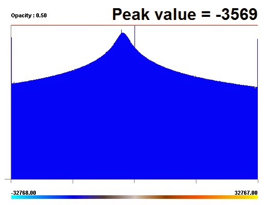
So in this example (from the Parihaka dataset), our peak value is -3569/1000 = -3.569.
If we calculate arctan (-3.569)= -74.347 degrees.
Then the χ = 90 - 74.347 = 15.65 degrees
Results
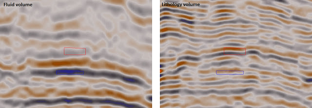
The image below shows the lithology and fluid volumes calculated on the Parihaka dataset (Taranaki basin, New Zealand). As expected, the area where the class III anomaly was identified in the Part 3 of the series shows a high amplitude in the fluid volume, while the amplitudes in the lithology volume are fairly uniform.
As mentioned this was the last in the series on AVO screening - if you have any feedback on how useful it has been please let us know.
Background reading
Avseth, P., Mukerji, T. & Mavko, G. (2010). Quantitative Seismic Interpretation (2nd edition). Cambridge Press, Cambridge, UK.
Castagna & Smith (1994). Comparison of AVO indicators: A modeling study. Geophysics, 59, 1849-1855.
Nam, N. & Fink, L. (2008). From Angle Stacks to Fluid and Lithology Enhanced Stacks. 7th International Conference on Petroleum Geophysics, Hyderabad.
Rutherford & Williams (1989). Amplitude-versus-offset variations in gas sands. Geophysics, 54, 680–688.
Simm & Bacon (2014). Seismic Amplitude. An Interpreters Handbook. Cambridge Press, Cambridge, UK.
Whitcombe, D.N, Connolly, P.A., Reagan, R.L. and Redshaw, T.C. (2002). Extended elastic impedance for fluid and lithology prediction. Geophysics, 67, 63–67.
