

One way to incorporate information from FMI logs into Geoteric is to classify fault by their trend (orientation along strike). This will allow the user to quickly correlate the orientation of open fractures/faults from FMI logs to the seismic volume, gaining a better understanding of the direction of these fractures/faults.
The input for this workflow is the Fault Detect volume, which is generated from the Fault Expression workflow. The Fault Detect volume captures the 3D fault/fracture network that is detected from the CMY blend of three edge attributes or from a single edge attribute. Below is a list of previous blog posts which detail the Fault Detect volume and an example case study:
- Fault Expression (video)
- CMY blends to Faults
- Fault Expression: A Basic step-by-step guide
- 7 tips for using GeoTeric's Fault Expression tool
- Correlating seismic faults with well based faults (video)
By creating a Fault Trend attribute, it is possible to classify faults or fractures according to their orientation/direction.
- Under the Reveal Tab, select Processes & Workflows which will then open the Batch Processor.
- Go to Processes >Faults>Fault Trends
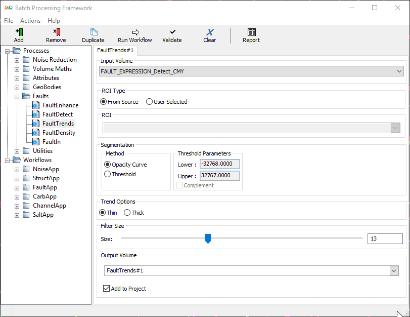
Figure 1: Batch Processor showing Fault Trends options
- The Input Volume must be the Fault Detect volume.
- Segmentation - Method will decide which values from the input volume you want to include in this process. This can be set by Threshold or by Opacity Curve. Threshold will require you to manually enter the data range values you wish to be included in the Fault Trend process, this allows you to filter out low confidence faults. Using the Opacity Curve, will allow you to interactively determine the values you wish to include (see following steps and images).
Note: If you are using the Opacity Curve method for Segmentation of the Fault Detect volume, the opacity curve must be open and on display in order for it to link to the process.
- To determine which fault trends to capture, in the main GeoTeric Project Tree, double click on the Fault Detect volume and then click on Opacity (Figure 2 – circled red) which will open the opacity window (Opacity Editor). The opacity curve can be manipulated by drawing on the opacity curve – depicted in the following images.
Tip: The Fault Detect volume defaults with the Body Spectrum Colour Bar, which associates colour with confidence. Red = higher confidence faults and Blue = lower confidence faults/noise. By segmenting the Fault Detect volume, this will allow you to select only the faults you want to include in the Fault Trends analysis and the noise/low confidence faults can be removed.
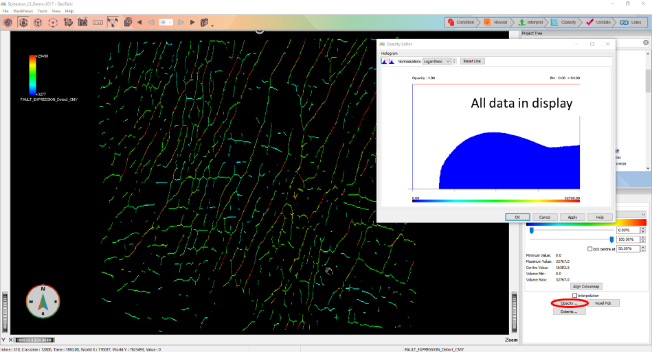
Figure 2: Fault Detect in main 3D window with no segmentation to Opacity Editor. Image is of a timeslice.
- In the Opacity Editor, to edit the opacity curve, hold down the left mouse button, a pencil will appear then drag to where you want to begin segmenting your data. Click apply to view segmentation in 3D viewer, all the faults to right of the red line (pictured below - Figure 3 ) will remain and all values to the left, will be removed.
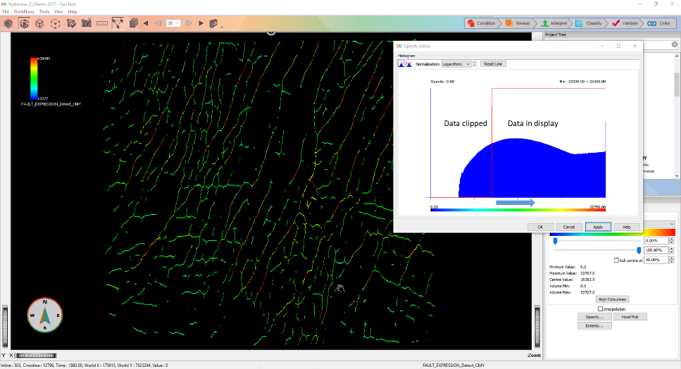
Figure 3: Fault Detect in main 3D window with segmentation (note only the faults with higher confidence are left in display). Image is of a timeslice.
NB: Even if you are not segmenting particular fault values, you should always remove the zero (black) values as this represents non-fault information which you do want to include in the Fault Trends.
Once you have edited the opacity curve to display the values (faults) you want in the Fault Trend volume, you can click Run Workflow in the Batch Processor.
Figure 4 – Batch Processing Framework, FaultTrendRotary default
The Fault Trend volume groups the faults into their dominant orientation – which will be coded by colour. All faults that share the same colour will have the same orientation. The default colour bar is the FaultTrendRotary, where North is associated with red.
The next step is to convert the Fault Trends Value into angles of degree in order to correlate to other geological data or if user want to compare the Fault Trends result to the orientation from FMI Log Analysis.
Access our original blog post here.
The conversion is done with the Parser. The Parser is located in the Batch Processing, under Volume Maths. The input volume is the newly created Fault Trends volume, this will be im1. If the input volume is a 16 bit data, the following equation can be used:
(im1>0)*(im1/182)
If the volume is 32 bit, please use this:
(im1>0)*(im1/11930464)
The resulting volumes will have a value range between 0 and 180. Zero represents the non-fault voxels. In order to correctly display the Fault Trends in degrees, use FaultTrendsRotary colour map. A rotary colourmap should always be used as the data with a value of 0 has the same trend as data with a value of 180.
When displaying the volume, in the properties panel, untick the interpolation box, so that you can see the true colour that changes according to trends.
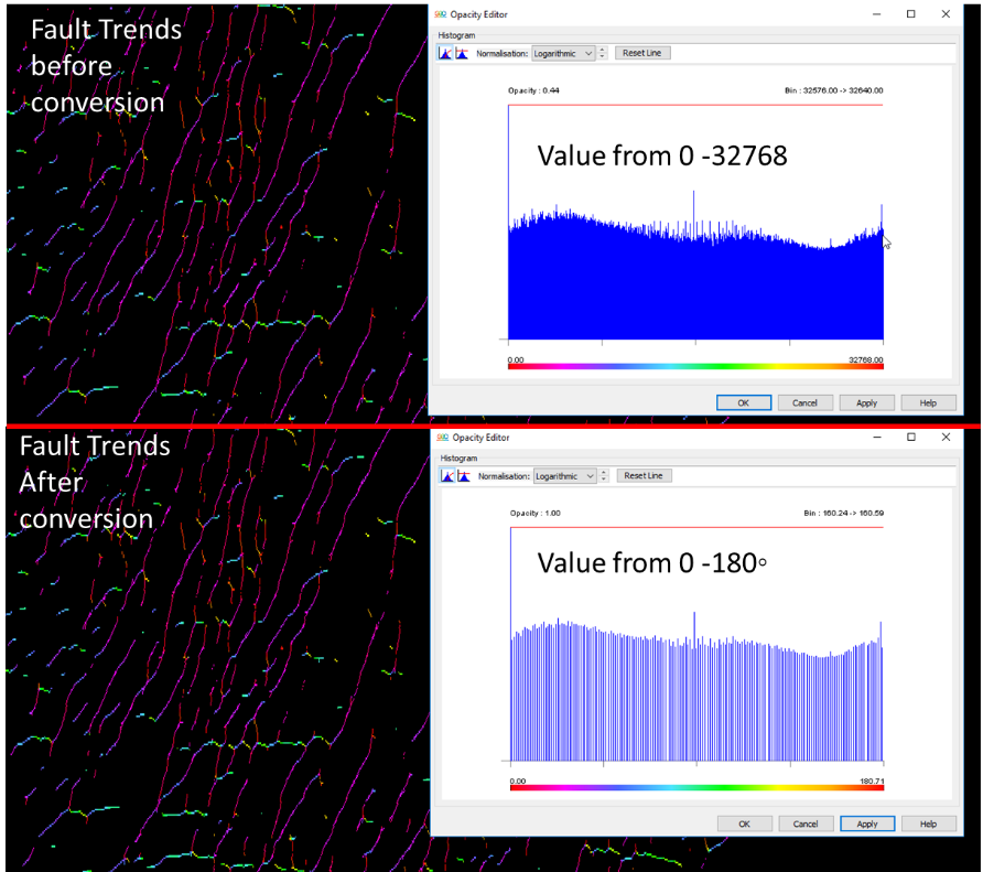
Figure 5: Fault Trends value that was converted into degree.
Tip: The colour corresponds to orientation, with red aligning with north, this will enable you to determine which colours relate to which directions, giving you a more comprehensive understanding of the different structural regimes in your region without having to interpret first.
So far, we have transformed the Fault Detect volume into different fault trends which are colour coded according to their angle. But what if the user would like to retain only a certain orientation and filter out the rest? The user can go through the process of segmenting the Fault Trends again, but choose the range of angles to display by using opacity or the threshold value.
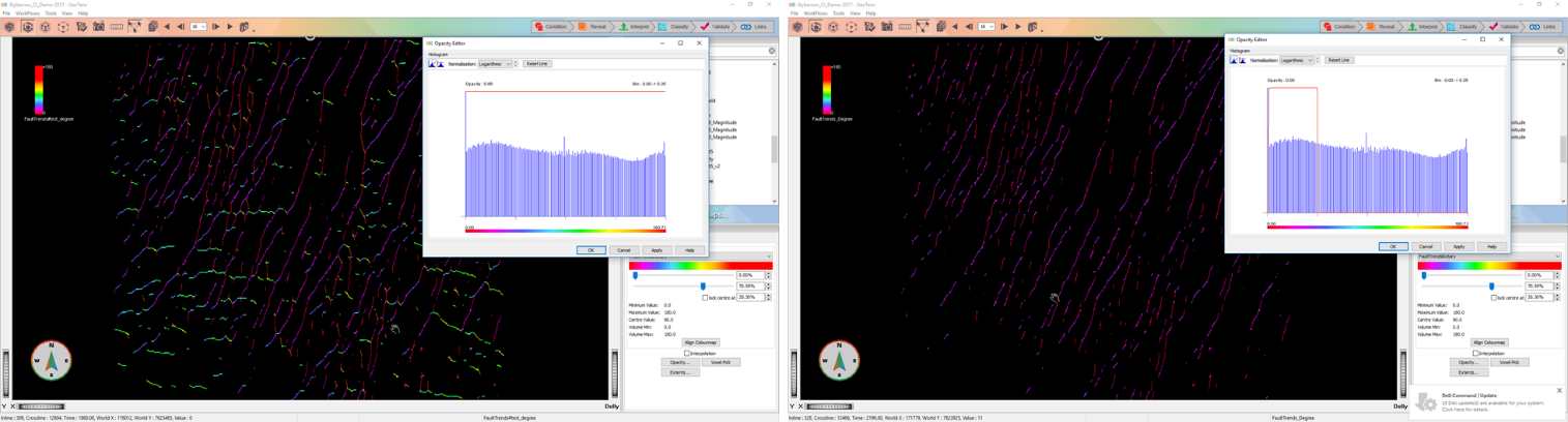
Figure 6:On the left image - Fault Trend without filtering. On the right image -Fault Trend for 0-45 degree only, everything else filtered out. Image is on a timeslice.
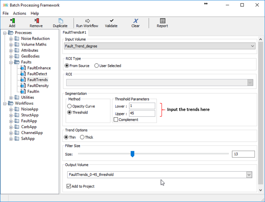
Figure 7: Instead of the opacity, you can use the threshold method and input the range of degrees you want. Both will give you almost the same result but the threshold method has higher accuracy.
Once the faults are displayed as angles and have been segmented to the users desired orientation, the Fault Density can be used to calculate the spatial distribution of fault/fracture within the seismic. In other words, the user can determine areas that have the highest number of occurring fault/fracture within the seismic. When used in combination with the Fault Trends workflow, the user can find the highest density of fault or fracture with a certain orientation anywhere within the seismic or in the reservoir interval.
NB: Dip and Azimuth volume are needed for Structural Oriented Fault Density calculation.
For example, in a fracture basement reservoir, one would be interested only to look for a certain fracture trends that can be associated with an open fracture. Whether the fractures are closed or open, this information can only be obtained from the FMI log analysis and by comparing and correlating both trends from logs and seismic, potential fracture or open fractures zones away from the borehole can be mapped.
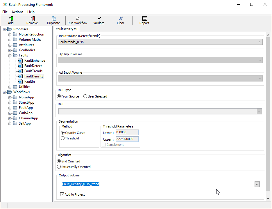
Figure 8: Input Fault Trends into Fault Density process.
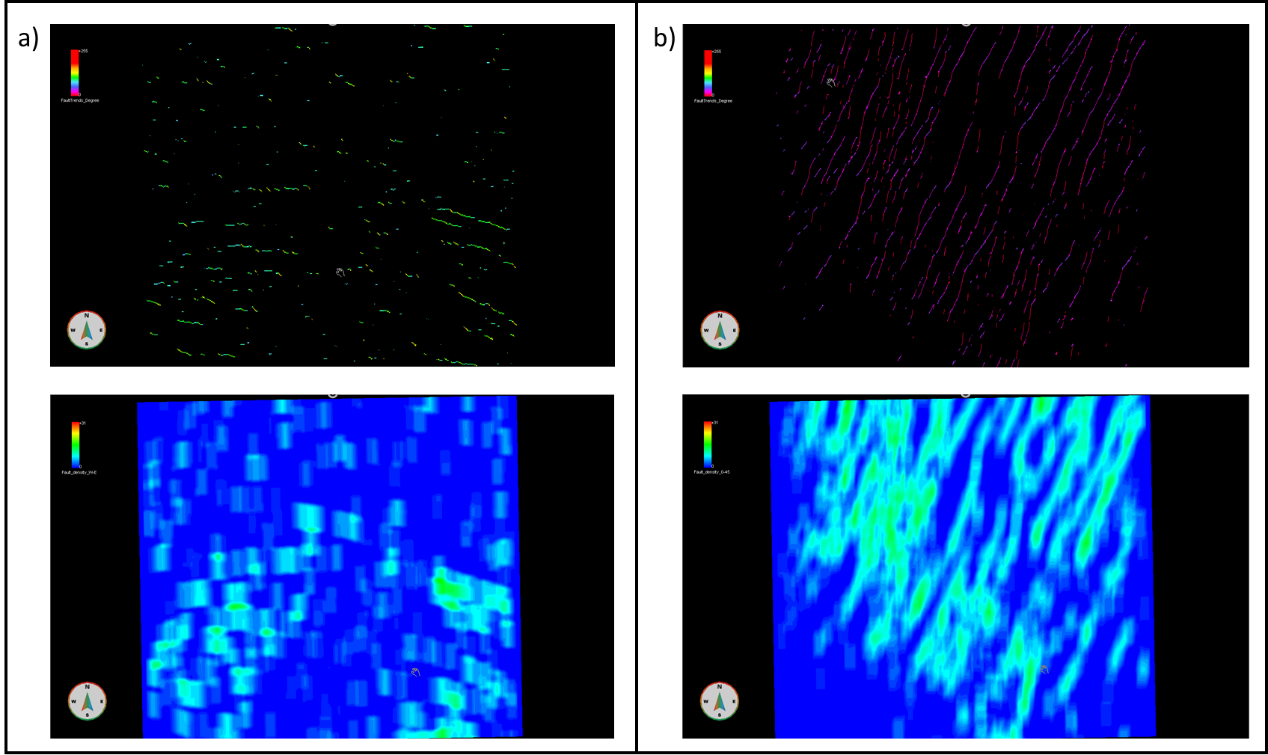
Figure 9: All 4 images are displayed on a time slice. a) Fault Trends which are oriented W-E and its Fault Density. b) Fault Trends oriented 0-45 (NE-SW) and its Fault Density.
